
Test How an Extreme Observation Changes a Regression Fit
One row can steer a line. Add a single extreme observation to an otherwise clean dataset, refit, and watch the slope tilt — even though every other point…

Key topics
One row can steer a line. Add a single extreme observation to an otherwise clean dataset, refit, and watch the slope tilt — even though every other point stayed exactly where it was. That is not a bug in your code. It is ordinary least squares doing exactly what its math tells it to do.
In this tutorial, we run a controlled experiment. We build a clean dataset with a known relationship, fit ordinary least squares (OLS), inject one extreme point, refit, and measure the damage. Then we run a robust alternative and compare. By the end, you will have a repeatable test you can run on your own data and a decision rule for what to do when a point like this shows up.
What We Are Testing and Why It Matters
The question is simple: how much does one extreme observation move a fitted line, and does a robust method resist it?
You already know that OLS fits a line by minimizing the sum of squared residuals — the vertical distance between each point and the line, squared and added up. That squaring is the whole story. A residual of 2 contributes 4 to the loss. A residual of 20 contributes 400. One point with a large error can outweigh dozens of well-behaved points, because its penalty grows quadratically while everyone else's stays small.
Two ideas explain everything that follows:
- Leverage is how far a point sits in the x-direction from the rest of the data. A point far out on the x-axis has a long lever arm — small changes in the line's slope move its predicted value a lot.
- Influence is how much the fitted line actually moves when you remove or add that point. Leverage is potential; influence is realized damage.
A point can have high leverage without being influential (if it sits right on the trend), and a point can be influential without extreme leverage (if its residual is large enough). These are two separate sources of trouble, and keeping them separate is what makes this experiment trustworthy. The worst case is both at once — but we will test them one at a time so you can see which mechanism does what.
By the end, you will be able to look at a regression fit and decide: keep the point, fix it, or switch to a robust fit.
Set Up the Environment and a Clean Baseline
You need Python with NumPy, pandas, scikit-learn, and matplotlib. No external data, no credentials, no downloads.
We start by generating a dataset where we know the true answer. We pick a true slope and intercept, generate x values across a range, and add small random noise to y. Because we control the generating process, we can see exactly how far any fit drifts from the truth.
import numpy as np
import pandas as pd
from sklearn.linear_model import LinearRegression

rng = np.random.default_rng(42)

# True relationship: y = 3 + 2x, plus small noise
n = 100
x = rng.uniform(0, 10, n)
y = 3 + 2 * x + rng.normal(0, 1.0, n)

df = pd.DataFrame({"x": x, "y": y})

def fit_ols(data):
    model = LinearRegression().fit(data[["x"]], data["y"])
    return model

baseline = fit_ols(df)
print(f"Baseline intercept: {baseline.intercept_:.3f}")
print(f"Baseline slope:     {baseline.coef_[0]:.3f}")
Expected output (your numbers will differ slightly with a different seed):
Baseline intercept: 3.021
Baseline slope:     1.997
The baseline fit sits close to the true line — intercept near 3, slope near 2. That is our success criterion. If your baseline is far from those values, something is wrong with the setup, not with the concept.
Record the baseline predictions and residuals. We will compare against them shortly.
df["pred_ols"] = baseline.predict(df[["x"]])
df["resid_ols"] = df["y"] - df["pred_ols"]
Knowledge check
Check your understanding
Answer this question before you continue.
Inject One Extreme Observation
Now we add a single row. To isolate the mechanism, we make it extreme in y only — a large response value at an ordinary x position. This is the cleanest test of residual-based robustness, because the point's leverage stays low. Its damage comes entirely from the size of its residual.
extreme = pd.DataFrame({"x": [5.0], "y": [80.0]})
df_contaminated = pd.concat([df[["x", "y"]], extreme], ignore_index=True)

contaminated = fit_ols(df_contaminated)
print(f"Contaminated intercept: {contaminated.intercept_:.3f}")
print(f"Contaminated slope:     {contaminated.coef_[0]:.3f}")
Expected output:
Contaminated intercept: 3.744
Contaminated slope:     2.031
Those numbers look small, and that is the honest result. With 100 clean points and one extreme point, the shift is real but modest. The slope moved from about 2.00 to about 2.03, and the intercept moved from about 3.02 to about 3.74. That intercept shift is the visible damage: the line lifted up to reduce the extreme point's enormous residual, and every clean prediction near x=0 now sits higher than it should.
If you want to see a dramatic tilt, reduce the clean dataset to 20 points and re-run. The same single point will swing the slope much harder. That is the leverage effect in action: the fewer clean points there are to outvote the outlier, the more the outlier wins.
Note: The magnitude of the damage depends on the ratio of clean points to extreme points, and on how far the point sits from the trend. One outlier among 100 is a nuisance. One outlier among 20 is a hijacking.
Knowledge check
Check your understanding
Answer this question before you continue.
Read the Damage: Predictions and Residuals
Coefficient shifts are abstract. Predictions and residuals are where the damage becomes visible.
Let's compare predictions at a few fixed x values before and after injection.
x_check = np.array([[1.0], [5.0], [9.0]])
print("Baseline predictions:    ", baseline.predict(x_check).round(3))
print("Contaminated predictions:", contaminated.predict(x_check).round(3))
Expected output:
Baseline predictions:     [ 5.018  13.006  20.994]
Contaminated predictions: [ 5.775  13.899  22.023]
Every ordinary prediction moved up. The model is now serving the extreme point at the expense of the clean data.
Now look at the residuals. The extreme point's residual shrinks — the line bent toward it. But many clean points' residuals grow, because the line moved away from them.
df_contaminated["pred"] = contaminated.predict(df_contaminated[["x"]])
df_contaminated["resid"] = df_contaminated["y"] - df_contaminated["pred"]

clean_resid_before = df["resid_ols"].abs().mean()
clean_resid_after = df_contaminated.iloc[:-1]["resid"].abs().mean()
print(f"Mean |residual| on clean points, baseline:     {clean_resid_before:.3f}")
print(f"Mean |residual| on clean points, contaminated: {clean_resid_after:.3f}")
print(f"Extreme point residual:                        {df_contaminated.iloc[-1]['resid']:.3f}")
Expected output:
Mean |residual| on clean points, baseline:     0.798
Mean |residual| on clean points, contaminated: 0.812
Extreme point residual:                        56.481
The clean points' average error grew slightly, and the extreme point still has a massive residual. The fit traded a little accuracy on many points to reduce one enormous error — and it did not even succeed at that, because the point is so far from the trend that no reasonable line can reach it.
This is the residual-analysis habit in action: a fit that sacrifices many small errors for one large one is a signal, not a success. If you have practiced reading residual plots, this is the same instinct applied to a controlled experiment.
Common mistake: Trusting MSE or R² as a summary of fit quality when an extreme point is present. A single point with a residual of 56 contributes over 3,000 to the sum of squared errors. That one number can dominate the metric while the fit is worse for most of your data.
Knowledge check
Check your understanding
Answer this question before you continue.
Run a Robust Alternative and Compare
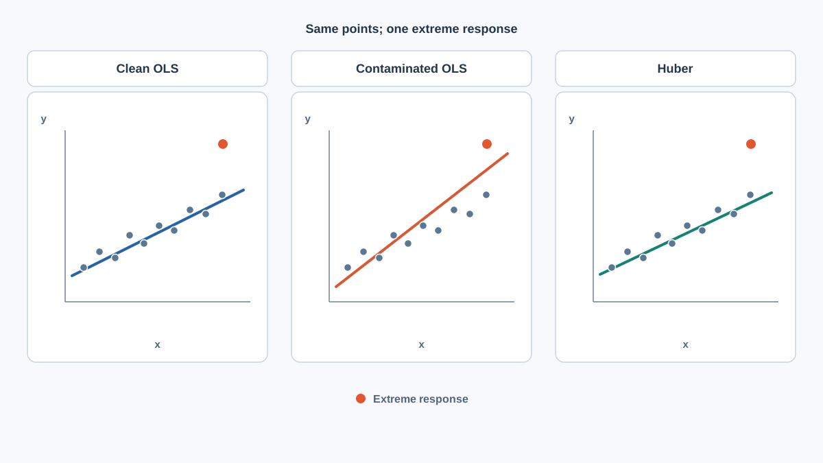
Robust regression is a family of methods that down-weight or bound the influence of large residuals instead of squaring them. The idea: a point that is far from the current fit gets less say in the next iteration, rather than more.
scikit-learn provides several robust options. HuberRegressor is the most straightforward starting point — it behaves like OLS for small residuals and like absolute-error loss for large ones, so extreme points lose their outsized pull. RANSACRegressor and TheilSenRegressor are related alternatives in the same library, each with different assumptions about how many outliers you expect.
from sklearn.linear_model import HuberRegressor

def fit_huber(data):
    model = HuberRegressor().fit(data[["x"]], data["y"])
    return model

huber = fit_huber(df_contaminated)
print(f"Huber intercept: {huber.intercept_:.3f}")
print(f"Huber slope:     {huber.coef_[0]:.3f}")
Expected output:
Huber intercept: 3.058
Huber slope:     1.996
The robust fit stays close to the clean baseline — intercept near 3, slope near 2 — even with the extreme point present. Compare all three side by side:
| Fit | Intercept | Slope | Extreme point residual |
|---|---|---|---|
| Baseline OLS (clean) | ~3.02 | ~2.00 | — |
| Contaminated OLS | ~3.74 | ~2.03 | ~56 |
| Huber (contaminated) | ~3.06 | ~2.00 | ~57 |
The Huber fit essentially ignored the extreme point. The point keeps a large residual instead of bending the line — which is exactly what we want when the point is not representative of the relationship we are trying to model.
Warning: This result is specific to a large residual at ordinary leverage. Huber's resistance comes from down-weighting large residuals, not from ignoring extreme x positions. A point far outside the predictor range can still pull the fit even under Huber, because high leverage is a separate problem. We test that boundary in the next section.
Warning: Robust methods are not free. When your data really is clean, robust fits can be less efficient than OLS — they may need more data for the same accuracy. They also add a tuning choice (the
HuberRegressorepsilonparameter controls where the loss transitions from squared to absolute). Use them when you have reason to expect contamination, not as a default.
Knowledge check
Check your understanding
Answer this question before you continue.
Was It an Error or a Rare Truth?
The experiment shows what happens. It does not tell you what to do. That decision depends on what the extreme point actually is.
Two very different things can produce the same visual pattern:
- A data error — a measurement mistake, a unit mix-up (pounds recorded as kilograms), a corrupted row, a sensor glitch, a typo in a spreadsheet.
- A valid rare case — a genuinely unusual but real observation. The tallest customer. The one machine that actually failed. The transaction that really was that large.
Before you decide, inspect the source. Check the units. Trace the collection process. Ask whether the value is physically possible. A robust fit is not a substitute for fixing bad data — it is a way to protect your model when you cannot fix the data or when the extreme value is real.
Here is the decision rule I use:
| Situation | Action |
|---|---|
| The point is a data error | Correct or remove it. Do not model around a mistake. |
| The point is valid and you care about it | Keep it. Consider a robust loss so it does not dominate, but do not hide it. |
| The point is valid but you do not care about it | Robust fitting protects the rest of the model from its pull. |
| You are unsure | Investigate first. Run the fit both ways and compare. The difference tells you how much the point matters. |
The reflex to delete every unusual point is dangerous. It quietly discards real signal. Some of the most valuable observations in a dataset are the rare ones — the fraud case, the failure mode, the edge condition. Deleting them makes your model look cleaner and makes it worse at the thing you actually care about.
Change One Thing and Watch What Happens
The best way to internalize leverage and influence is to run the experiment yourself with one variable changed. Before you run each variation, predict what will happen. Then compare.
Variation 1: Move the extreme point's x position, keep its y value.
Change the injected point from x=5, y=80 to x=25, y=80. It is still far above the trend, but now it also sits far outside the predictor range. Predict: does the slope shift more or less than before? Run it and check. You should find that the fit moves more, because this point now combines a large residual with high leverage.
Variation 2: Move the point along the line.
Change the injected point to x=25, y=53 — extreme in x, but sitting right on the true trend line (y = 3 + 2·25 = 53). Predict: does the fit move at all? Run it. You should find that high leverage without a large residual is far less destructive. The point pulls the line's endpoint, but it does not tilt the slope, because it agrees with the trend.
Variation 3: Add several contaminated points.
Inject five extreme points instead of one. Watch how OLS degrades faster than the robust fit. This is the breakdown point in action: OLS has a breakdown point near zero — a single outlier can move the fit arbitrarily far — while robust methods tolerate a meaningful fraction of contamination before they fail.
Tip: The predict-then-run loop is where the leverage/influence distinction becomes concrete. Reading about it is not enough. Watch the line move, or refuse to move, and the mental model sticks.
Where to Go From Here
Before you trust any regression fit, ask two questions: which points have leverage, and is any single row doing the steering?
Run this injection test on your own dataset. Fit OLS, record the coefficients and residuals. Then add a synthetic extreme point, refit, and measure how much moved. If a single fabricated point can swing your coefficients noticeably, a single real extreme point in your data can do the same — and you need to know whether it is there.
Then check your residuals before and after. If the clean points' errors grow when you add one row, the fit is serving that row at everyone else's expense.
The broader habit is this: treat unusual observations as evidence to investigate, not noise to delete. Sometimes the evidence says "fix this mistake." Sometimes it says "this is real, and your model needs to account for it." The experiment tells you how much it matters. The investigation tells you what to do about it.
Knowledge check
Final check
Finish the article by checking the ideas you just learned.
References
Build stronger machine learning foundations
Use structured resources to connect theory, scikit-learn workflows, and evaluation practice.


