
Compare Polynomial Degrees With Leakage-Safe Validation
Fit degree 1 through 9, watch training error fall to almost zero, and pick degree 9. That is the trap. Training error measures how well a model remembers…

Key topics
Fit degree 1 through 9, watch training error fall to almost zero, and pick degree 9. That is the trap. Training error measures how well a model remembers the data it already saw. It says almost nothing about the data it has not seen yet.
So we are going to run a small, controlled experiment. We will compare a bounded set of polynomial degrees using a leakage-safe workflow, read the training-versus-validation behavior, and choose a degree for a reason we can defend. The code is short. The judgment is the real work.
What We Are Actually Comparing
You already know the mechanism from polynomial feature expansion: PolynomialFeatures turns one input column into powers of that input, and a linear model fits coefficients on those powers. The model is still linear in its parameters. The curve comes from the features, not from a nonlinear solver.
That means the decision variable here is simple: the degree. Everything else stays fixed — same model family, same metric, same data split, same random seed. Change one thing, hold the rest constant, and the comparison is controlled.
Keep the search bounded. Degrees 1, 2, 3, 5, and 9 are enough to see the shape of the tradeoff. A sweep to 20 adds noise, cost, and numerical trouble without teaching you anything new.
Before writing code, state what success looks like:
- A validation curve you can actually read.
- A chosen degree with a stated reason.
- A visible gap between training and validation error that you can explain.
And state the non-goal plainly: this experiment does not prove which degree is right for your real dataset. It teaches you the workflow for finding out.
Knowledge check
Check your understanding
Answer this question before you continue.
Prerequisites and Setup
One short bridge, then we move. You should already know that feature expansion creates curvature and that raising the degree raises variance. If that is shaky, read the polynomial regression concept first, then come back.
You need Python with NumPy, pandas, scikit-learn, and matplotlib. No external services, no credentials, no downloads.
import numpy as np
import pandas as pd
import matplotlib.pyplot as plt

from sklearn.pipeline import make_pipeline
from sklearn.preprocessing import PolynomialFeatures
from sklearn.linear_model import LinearRegression
from sklearn.model_selection import train_test_split, KFold, cross_validate
from sklearn.metrics import mean_squared_error, make_scorer
Now the data. We generate a small 1-D regression set with a known underlying curve plus Gaussian noise, using a fixed seed so your output matches mine.
rng = np.random.default_rng(0)

def true_curve(x):
    return 0.5 * x**3 - x**2 + 2 * x + 1

X = rng.uniform(-3, 3, size=120).reshape(-1, 1)
y = true_curve(X.ravel()) + rng.normal(0, 3.0, size=120)
Why synthetic first? Because we control the true function. We know the signal. So when the model stops learning signal and starts memorizing noise, we can see it happen instead of guessing.
Build the Leakage-Safe Pipeline
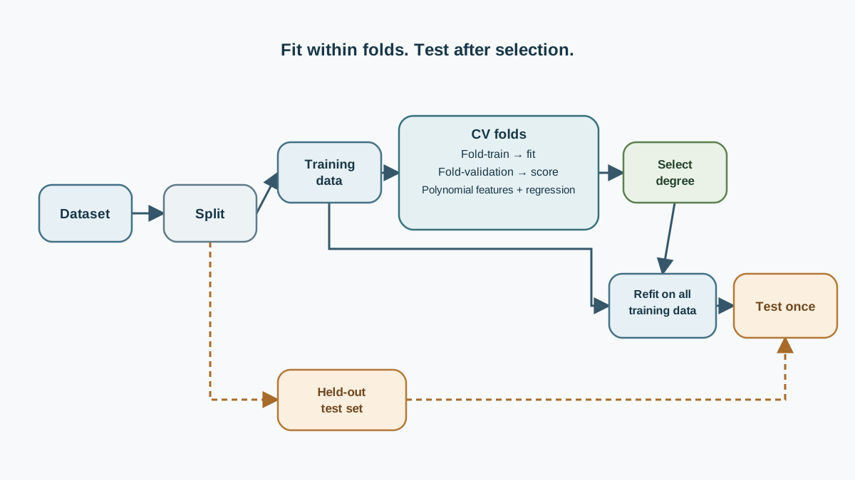
Here is the smallest correct implementation:
def make_model(degree):
    return make_pipeline(
        PolynomialFeatures(degree=degree, include_bias=False),
        LinearRegression(),
    )
Two steps, wrapped so they behave as one estimator. That wrapping is the whole point.
Now the leakage rule, stated precisely, because it is easy to overstate. PolynomialFeatures is a deterministic transform: it computes powers of each input value. It does not estimate a mean, a scale, a category encoding, or any statistic from your data. In this one-feature example, expanding the full dataset before splitting would not leak the validation targets, and it would not "learn the shape" of the validation range.
So why wrap it in a pipeline at all? Because the pipeline is the pattern that keeps you safe the moment a step does learn from data. Standardization, imputation, target encoding, and PCA all estimate parameters from the rows they see. If you fit those on the full dataset and then split, the transform has already absorbed information from the validation rows, and your scores come back optimistic. The pipeline clones and refits every step inside each fold, so each transform learns only from that fold's training rows and is applied to that fold's validation rows. No information crosses the boundary.
Common mistake: fitting a learned transform — a scaler, an imputer, an encoder — on the full dataset before splitting. The symptom is validation scores suspiciously close to training scores, or scores that collapse the moment you switch to a fresh split. Fix the pipeline order, not the metric.
One detail worth keeping consistent: include_bias=False here because LinearRegression fits its own intercept. Whatever you choose, choose it once and apply it to every degree, or the comparison stops being fair.
Knowledge check
Check your understanding
Answer this question before you continue.
Run the Degree Comparison
Now the experiment. Loop over the bounded degree list, run k-fold cross-validation on the training set, and collect mean training error and mean validation error.
degrees = [1, 2, 3, 5, 9]

X_train, X_test, y_train, y_test = train_test_split(
    X, y, test_size=0.25, random_state=0
)

cv = KFold(n_splits=5, shuffle=True, random_state=0)
scoring = {
    "train": make_scorer(mean_squared_error, greater_is_better=False),
    "val": make_scorer(mean_squared_error, greater_is_better=False),
}

rows = []
for degree in degrees:
    model = make_model(degree)
    scores = cross_validate(
        model, X_train, y_train, cv=cv, scoring=scoring,
        return_train_score=True,
    )
    train_mse = -scores["train"].mean()
    val_mse = -scores["val"].mean()
    val_std = scores["val"].std()

    final = make_model(degree).fit(X_train, y_train)
    test_mse = mean_squared_error(y_test, final.predict(X_test))

    rows.append({
        "degree": degree,
        "train_mse": train_mse,
        "val_mse": val_mse,
        "val_std": val_std,
        "test_mse": test_mse,
    })

results = pd.DataFrame(rows)
print(results.round(2))
Two details make this code honest. First, return_train_score=True is what actually produces training-fold scores; without it, scores["train"] would not exist and you would be reading validation numbers under a training label. Second, val_std is a standard deviation, so it stays positive — only the error means get negated, because greater_is_better=False flips the sign of the scorer.
Use at least 5 folds, and report the spread across folds alongside the mean. A single number hides how unstable a high degree really is.
The test set was never touched during selection. It is the final check, not the selection tool. That distinction matters, and we will come back to it.
Your table should look roughly like this:
| degree | train_mse | val_mse | val_std | test_mse |
|---|---|---|---|---|
| 1 | high | high | small | high |
| 2 | lower | lower | small | lower |
| 3 | low | lowest | small | low |
| 5 | very low | rising | larger | rising |
| 9 | near zero | high | large | high |
The exact numbers depend on the seed and the noise. The shape is what you read. Plot training and validation error against degree:
plt.plot(results["degree"], results["train_mse"], marker="o", label="train")
plt.plot(results["degree"], results["val_mse"], marker="o", label="validation")
plt.xlabel("polynomial degree")
plt.ylabel("mean squared error")
plt.legend()
plt.show()
Read the curve, not one row. The useful signal is where validation error stops falling while training error keeps dropping.
Knowledge check
Check your understanding
Answer this question before you continue.
Read the Training-Validation Gap
The gap between the two curves is the diagnosis. Absolute error is not.
Low degree. Both errors are high and close together. The model is too rigid to capture the curve. That is underfitting, and adding data will not fix it.
Middle degree. Validation error sits at its minimum, training error is modestly higher. The model is capturing signal without chasing noise. This is the region you want.
High degree. Training error approaches zero, validation error climbs, and fold-to-fold spread widens. The model is fitting noise, and it is becoming unstable — different folds disagree about what the right answer is.
A model with low training error and a large gap is not a better model. It is a more confident memorizer.
Boundary caution: polynomial curves can oscillate sharply near the edges of the data range. Error measured only in the middle of the range can understate the problem. If your data has sparse edges, check predictions there separately.
Knowledge check
Check your understanding
Answer this question before you continue.
Failure Modes and Debugging Signals
Keep this list next to your output. Each symptom points at a specific fix.
Leakage. Validation scores suspiciously close to training scores, or scores that collapse on a fresh split. Check whether any learned transform was fit outside the pipeline. Fix the pipeline order, not the metric.
Numerical instability. Very high degrees produce huge feature values and ill-conditioned fits. Coefficients swing wildly between folds. That is a signal to stop increasing degree, not to add more folds.
Selection on the test set. If you pick the degree by test error, the test set is no longer a test set. Choose with cross-validation, then report once.
Single-split luck. One train/test split can make a bad degree look good. Cross-validation plus a final held-out check reduces that risk.
Over-reading one dataset. A degree that wins on this synthetic curve may lose on real data with different noise, range, or feature count. The workflow transfers. The winning number does not.
One Modification Worth Trying
Copying the code teaches you syntax. Changing one variable teaches you judgment.
Raise the noise level, shrink the number of training rows, or narrow the input range — one at a time — and rerun the same comparison. Watch how the best degree moves. With more noise or less data, the validation minimum usually shifts toward simpler models. That shift is the lesson: complexity is not a property of the model alone. It is a relationship between the model and the data you have.
Then add a regularized variant. Swap LinearRegression for Ridge in the same pipeline and compare where the validation curve bottoms out. Degree is one lever on complexity. Regularization is another. They trade against each other, and the right setting depends on the data, not on a rule of thumb.
Where This Leaves You
Choose the degree at the validation minimum. Confirm it once on untouched data. If the answer requires a very high degree to compete, treat that as evidence that polynomial regression may be the wrong tool — spline-based features are often a better fit for the same problem, with better numerical behavior and less boundary oscillation.
The value of this experiment is not the winning number. It is the workflow: hold everything fixed, expand inside the fold, read the gap, and let the validation curve make the argument. Run it once on your own data, change one variable, and run it again. That second run is where the intuition actually forms.
Knowledge check
Final check
Finish the article by checking the ideas you just learned.
References
Build stronger machine learning foundations
Use structured resources to connect theory, scikit-learn workflows, and evaluation practice.


