Compare Ridge and Lasso Coefficients With a Controlled Scikit-Learn Experiment

You fit ridge, you fit lasso, lasso wins by a hair, and you quietly file away "lasso is better." That conclusion is a coin flip wearing a lab coat. One split, one alpha, one score is not evidence — it is a single roll of the dice. This tutorial builds the experiment that actually answers the question: a fixed split, a shared penalty grid, and two coefficient paths you can read with your own eyes.

By the end you will have a runnable script that sweeps regularization strength for both models, a table of nonzero coefficients, and two plots that make shrinkage and sparsity visible. The deliverable is not a winner. It is a setup you trust and a picture you understand.

What a Fair Ridge-vs-Lasso Comparison Actually Requires

Before writing a line of code, decide what would make the comparison valid — and what would quietly invalidate it.

Four conditions do the heavy lifting:

• Same rows, both models. Ridge and lasso must train on identical training rows and be scored on identical test rows. Different splits mean you are comparing datasets, not penalties.
• Same feature scaling. Both penalties are scale-sensitive. If one model sees standardized features and the other does not, the coefficients are not comparable.
• A shared alpha grid for the path plot. Sweep the same penalty strengths for both models so you can watch each estimator's response over the same range. This makes the coefficient paths visually comparable. It does not make each ridge point and each lasso point a matched-strength comparison — more on that below.
• Leakage-safe evaluation. Fit the scaler on training data only, then apply it to the test set. Scaling on the full dataset before splitting lets test-set statistics bleed into training — a small leak that inflates your score and flatters whichever model you ran second.

You already know the mechanism from the prerequisite intuition: ridge adds an L2 penalty, lasso adds an L1 penalty. Here we stop reasoning about that and start measuring it. The success criteria are concrete: a coefficient path per model, a count of nonzero coefficients at each alpha, and a final held-out score for each model after alpha is chosen properly.

Set Up the Data and the Leakage-Safe Split

You need scikit-learn, NumPy, pandas, and matplotlib. No credentials, no external services.

We will use the diabetes dataset — a small regression dataset with several correlated features, which gives both shrinkage and sparsity something to act on.

import numpy as np
import pandas as pd
from sklearn.datasets import load_diabetes
from sklearn.model_selection import train_test_split
from sklearn.preprocessing import StandardScaler

data = load_diabetes()
X = pd.DataFrame(data.data, columns=data.feature_names)
y = data.target

X_train, X_test, y_train, y_test = train_test_split(
    X, y, test_size=0.2, random_state=42
)

scaler = StandardScaler().fit(X_train)
X_train_s = scaler.transform(X_train)
X_test_s = scaler.transform(X_test)

print(X_train_s.shape, X_test_s.shape)
print(y_train.mean().round(1), y_test.mean().round(1))

Expected shapes are roughly (353, 10) and (89, 10). The target means should be close to each other; if they diverge wildly, your split is unlucky and worth re-seeding.

Warning: The scaler is fit on X_train only. Fitting it on the full X before splitting is the most common beginner leak in this experiment. It looks harmless. It is not.

Sweep Alpha and Record Coefficients for Both Models

Now the core loop. Build one log-scale alpha grid, fit both models at every value, and store the coefficients plus the training error. We deliberately do not touch the test set here — this loop is for watching coefficient behavior, not for scoring.

from sklearn.linear_model import Ridge, Lasso
from sklearn.metrics import mean_squared_error

alphas = np.logspace(-3, 2, 40)
rows = []

for a in alphas:
    for name, model in [("ridge", Ridge(alpha=a)), ("lasso", Lasso(alpha=a, max_iter=10000))]:
        model.fit(X_train_s, y_train)
        coefs = model.coef_
        train_err = mean_squared_error(y_train, model.predict(X_train_s))
        rows.append({
            "model": name,
            "alpha": a,
            "nonzero": int(np.sum(np.abs(coefs) > 1e-8)),
            "train_mse": train_err,
            "coefs": coefs,
        })

results = pd.DataFrame(rows)

Two things to notice.

First, the alpha conventions differ. Scikit-learn's lasso objective includes a 1/n_samples factor that ridge's does not. That means an alpha of 1.0 in Ridge is not the same penalty strength as an alpha of 1.0 in Lasso. This is a documented convention, not a bug. It is exactly why a shared grid is useful for plotting paths over a range — and why you should not read a shared-grid point as "equal penalty strength."

Second, the success criterion is visible in the table. Ridge coefficients should shrink smoothly as alpha grows. Lasso coefficients should drop to exact zeros. Print a compact view:

summary = results[results["alpha"].isin(alphas[::8])]
print(summary[["model", "alpha", "nonzero", "train_mse"]].to_string(index=False))

You should see ridge's nonzero count stay pinned at 10 while lasso's falls toward zero. That single column is the difference between the two penalties, rendered as an integer.

Read the Coefficient Paths

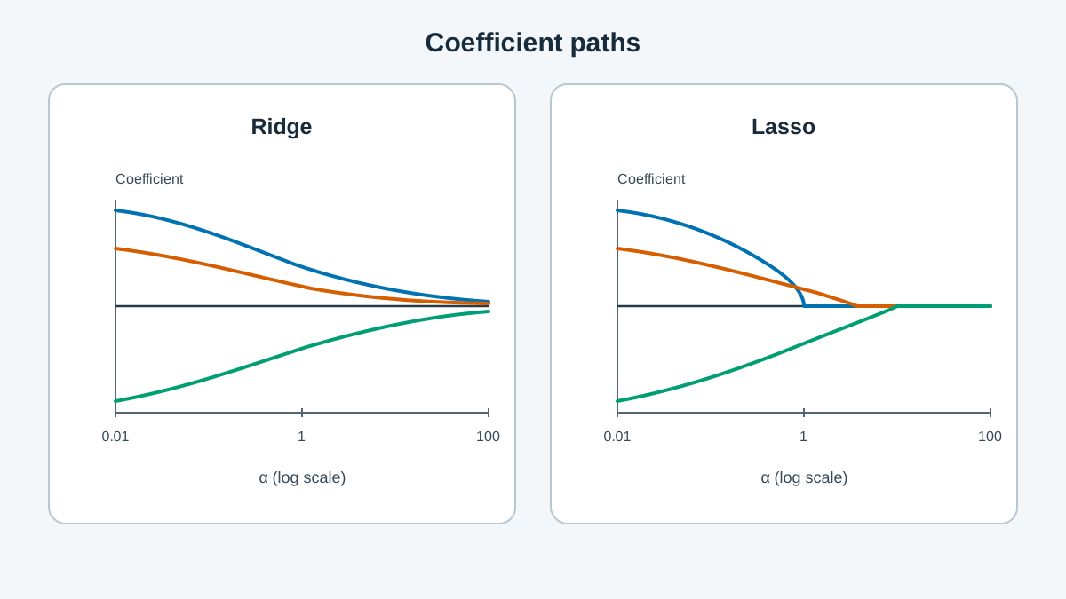
Numbers in a table are useful. Lines on a plot are memorable.

import matplotlib.pyplot as plt

fig, axes = plt.subplots(1, 2, figsize=(12, 5), sharey=True)

for ax, name in zip(axes, ["ridge", "lasso"]):
    subset = results[results["model"] == name]
    coef_matrix = np.vstack(subset["coefs"].values)
    for j in range(coef_matrix.shape[1]):
        ax.plot(subset["alpha"].values, coef_matrix[:, j], linewidth=1)
    ax.set_xscale("log")
    ax.set_title(name)
    ax.set_xlabel("alpha")
axes[0].set_ylabel("coefficient value")
plt.tight_layout()
plt.show()

Two shapes, two stories.

Ridge: every line bends toward zero as alpha grows, but none of them ever touches it. Shrinkage without elimination. The features stay in the model, just quieter.

Lasso: lines hit exactly zero at different alpha values. The order in which they drop is the sparsity story — and it is worth annotating the alpha where the first coefficient dies.

This is the L1-versus-L2 geometry made visible. The L1 constraint has corners, and coefficients can land exactly on them. The L2 constraint is smooth, so coefficients approach zero without arriving. You derived that in the prerequisite theory. Here you watch it happen.

Choose Alpha With Cross-Validation, Then Score Once

Here is the part that separates a real experiment from a demo. The coefficient paths above are exploratory — they show behavior, not performance. To compare held-out performance fairly, alpha must be chosen inside the training data, and the test set must be used exactly once, at the end.

from sklearn.linear_model import RidgeCV, LassoCV

ridge_cv = RidgeCV(alphas=alphas, cv=5).fit(X_train_s, y_train)
lasso_cv = LassoCV(alphas=alphas, cv=5, max_iter=10000).fit(X_train_s, y_train)

for name, model in [("ridge", ridge_cv), ("lasso", lasso_cv)]:
    test_mse = mean_squared_error(y_test, model.predict(X_test_s))
    print(f"{name}: alpha={model.alpha_:.4f}  test_mse={test_mse:.1f}")

Each model now gets its own alpha, chosen by 5-fold cross-validation on the training rows. The test set never influenced that choice. The printed test_mse is the first and only time the test set is used — and it is a genuine held-out estimate.

If you want to see the full error curves across alpha, plot them from cross-validated training scores, not from test scores:

from sklearn.model_selection import cross_val_score

for name, ModelClass in [("ridge", Ridge), ("lasso", Lasso)]:
    cv_means = [
        cross_val_score(ModelClass(alpha=a, max_iter=10000), X_train_s, y_train,
                        cv=5, scoring="neg_mean_squared_error").mean()
        for a in alphas
    ]
    plt.plot(alphas, -np.array(cv_means), label=name)
plt.xscale("log")
plt.xlabel("alpha")
plt.ylabel("cross-validated MSE (training folds)")
plt.legend()
plt.show()

Expect a U-shape for each model. Too little penalty and the model overfits; too much and it underfits. The minimum of each curve is the best alpha for that model on this data — not a universal best alpha, and not a matched-strength comparison between the two.

Common mistake: Computing test MSE for every alpha and picking the minimum. That turns the test set into a second training set. Your "held-out" score is now optimistic, and the model you selected was chosen partly by the data you claimed to hold out. Choose alpha with cross-validation on training folds. Score once.

Why Zero Coefficients Are Not Feature Discovery

A zero coefficient means one thing: given the other features in this model at this alpha, this feature did not earn its place. It does not mean the feature is irrelevant in the world.

With correlated predictors, lasso arbitrarily keeps one and zeroes its near-duplicates. Rerun with a different seed or split and the survivor can change. The sparsity is a property of the fitted model, not a claim about the data-generating process.

What actually changes which model looks better:

• Feature correlation structure. When predictors are highly correlated, lasso tends to pick one and zero its near-duplicates, while ridge spreads weight across all of them. Research on regularization benchmarks shows lasso's advantage shrinking or reversing in high-correlation and under-determined regimes.
• Sample-to-feature ratio. With few samples per feature, ridge is the safer default.
• Whether the true model is sparse. If only a handful of features genuinely matter, lasso's structure matches reality. If most features contribute a little, ridge does.

My rule: treat zeroed coefficients as a hypothesis to test on fresh data, never as a finished feature-selection result. If you want to act on sparsity, validate it out of sample.

Common mistake: Picking the features lasso zeroed and refitting ordinary least squares on the same data. That reuses the test information and produces an optimistic score that will not survive fresh data.

Modify the Experiment: Change One Thing

The lesson lives in the follow-up. Pick one change and rerun:

• Add near-duplicate features. Duplicate a column with small noise. Watch which one lasso keeps and whether held-out error moves at all.
• Shrink the training set. Drop to 50 training rows. Watch the two cross-validated curves separate as data gets scarce.
• Change the CV fold count. Move from 5 folds to 10. Watch the chosen alphas shift — a reminder that even cross-validated selection has variance.

Write down what changed and what stayed the same. That record — not the final score — is the actual lesson.

Note: This experiment shows behavior on one dataset and one split. It does not establish a general rule about ridge versus lasso. Anyone who claims otherwise from a single run is selling you a coin flip.

The next practical step is wrapping this whole sweep into a scikit-learn Pipeline so scaling and model selection travel together, then using GridSearchCV to tune alpha and any preprocessing choices in one leakage-safe object. That turns a one-split observation into a decision you can defend.