Fit and Evaluate Linear Regression With Scikit-Learn

A model that fits is not yet a model you can trust. Fitting takes one line. Trust takes a split, a reading of the numbers, and a look at where the errors land.

You already know what a line of best fit is. You know that linear regression picks the line minimizing the sum of squared errors, and that the gap between a real value and the predicted value is a residual. If any of that feels shaky, the first-principles article covers the derivation; here we assume it and move to the keyboard.

The goal of this tutorial is narrow and practical: build a leakage-conscious workflow in scikit-learn, read what the fitted model is telling you, and check whether it holds up on data it has never seen. By the end you will have a script you can point at your own dataset.

What You Need Before You Fit

You need Python with scikit-learn, numpy, pandas, and matplotlib. If scikit-learn is missing:

pip install scikit-learn

The mental model is small. A scikit-learn model is an estimator: an object that learns from data through a consistent interface. You instantiate it, call .fit(X, y), then call .predict(X_new) on new rows. For regression you can also call .score(X, y) to get a quick fit measure. That contract is the same whether you are running linear regression or a gradient-boosted tree, which is why learning it once pays off across the whole library.

One shape rule trips up nearly every beginner: X must be 2D, even when you have a single feature. A column of 100 values is shape (100,); scikit-learn wants (100, 1). If you pull a single column out of a DataFrame with df["rooms"], you get a 1D Series. Use df[["rooms"]] to keep it 2D.

The habit that prevents most beginner pain: split the data before you look at it, and never let the test rows influence any object you fit. We will do that first, before touching the model.

Split First, Fit Second

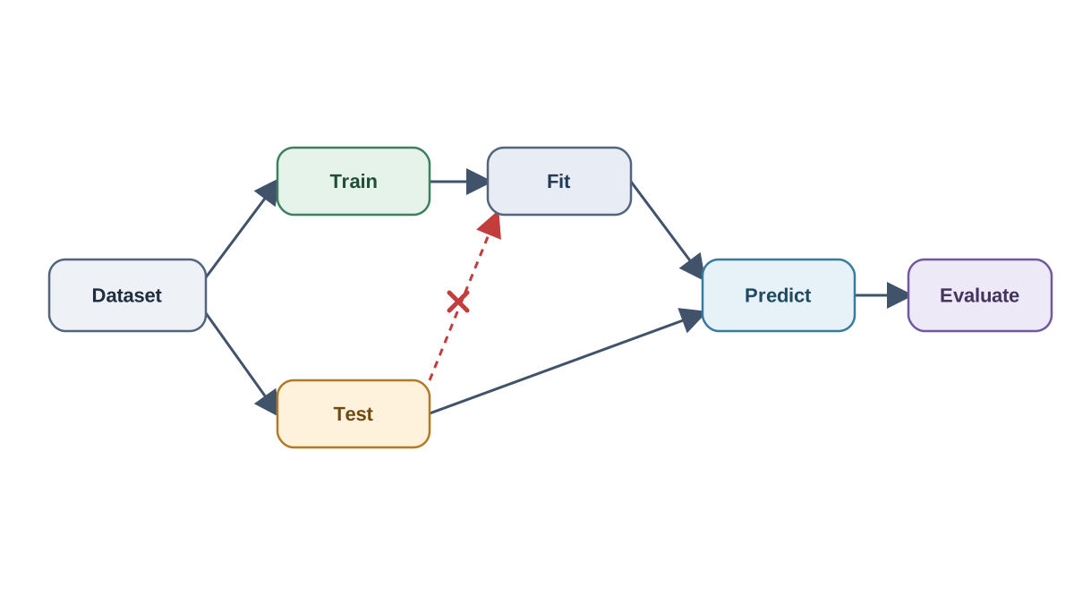
The order matters more than the ratio. A 70/30 split is fine; a leaky 70/30 split is not.

import numpy as np
import pandas as pd
from sklearn.model_selection import train_test_split

rng = np.random.default_rng(42)
n = 200
X = pd.DataFrame({
    "size": rng.normal(1500, 400, n),
    "age": rng.normal(20, 8, n),
})
y = 50 + 0.12 * X["size"] - 1.5 * X["age"] + rng.normal(0, 15, n)

X_train, X_test, y_train, y_test = train_test_split(
    X, y, test_size=0.2, random_state=42
)

The random_state makes the split reproducible. Without it, every run gives you a different test set, and you cannot tell whether a score changed because of your code or because of the shuffle.

Why split before scaling, imputing, or selecting features? Because anything fitted on the full dataset has already seen the test rows. If you compute the mean of a column across all rows and use it to fill missing values, that mean carries information from the test set into training. The model gets a small peek at the answers. That is data leakage.

The symptom is a test score that looks great and then collapses when you collect genuinely new data. The model was not better; it was just better informed than it should have been.

Note: Keep the test set untouched until the final evaluation. Use it once. If you tune against it repeatedly, it stops being a test set and becomes a second training set with extra steps.

Fit the Model and Read the Numbers

Now the fitting step, which really is one line.

from sklearn.linear_model import LinearRegression

model = LinearRegression()
model.fit(X_train, y_train)

coefs = pd.Series(model.coef_, index=X_train.columns)
print(coefs)
print(f"intercept: {model.intercept_:.2f}")

LinearRegression performs ordinary least squares. fit_intercept=True is the default, meaning the model estimates an intercept term. Setting it to False forces the line through the origin and assumes your data is centered; unless you have a specific reason, leave it on.

Wrapping model.coef_ in a pandas Series with X_train.columns as the index is the small move that makes coefficients readable. Instead of an anonymous array, you get one labeled value per feature, in the same order as your columns. If the labels do not match what you expected, you have caught a column-ordering bug before it poisoned your interpretation.

With the fixed seed above, the printed output lands close to:

size       0.12
age       -1.51
intercept: 51.4

Read the size coefficient in context: holding age fixed, a one-square-foot increase in size is associated with about a 0.12-unit increase in the predicted target. The age coefficient says the same thing in reverse — each additional year is associated with roughly a 1.5-unit drop, holding size fixed. The intercept is the predicted target when both features are zero, which here is outside the realistic range of the data and mostly serves as a mathematical anchor.

That reading is a statement about the fitted model, not about the world. Three reasons show up constantly:

• Correlated features. If two features move together, the model can shift weight between them almost arbitrarily. The individual coefficients become unstable even when predictions stay accurate.
• Omitted variables. A feature you did not include may be driving both the target and one of your inputs. The coefficient absorbs that influence and reports it as if it belonged to the feature you did include.
• Measurement error. Noisy inputs bias coefficients toward zero, sometimes substantially.

There is also a practical reading problem: if features are on different scales, coefficient magnitudes are not comparable. A coefficient of 0.12 for size in square feet and -1.5 for age in years tells you nothing about which feature "matters more" until you standardize them.

Before trusting the model on real data, run a sanity check on synthetic data where you know the answer.

rng = np.random.default_rng(0)
X_syn = rng.normal(size=(500, 2))
y_syn = 3.0 + 1.0 * X_syn[:, 0] + 2.0 * X_syn[:, 1] + rng.normal(0, 0.1, 500)

check = LinearRegression().fit(X_syn, y_syn)
print(check.coef_, check.intercept_)

You should see coefficients near [1.0, 2.0] and an intercept near 3.0. The small drift comes from the noise you added. Watching the model recover a known answer is the cheapest way to confirm you understand what the attributes mean before you point the same code at data whose true coefficients you will never see.

Predict, Then Score on Held-Out Data

With the model fitted on training rows, generate predictions for the test rows and compare.

from sklearn.metrics import mean_squared_error, r2_score

y_pred = model.predict(X_test)
mse = mean_squared_error(y_test, y_pred)
rmse = np.sqrt(mse)
r2 = r2_score(y_test, y_pred)

print(f"RMSE: {rmse:.2f}")
print(f"R2:   {r2:.3f}")
print(f"Train R2: {model.score(X_train, y_train):.3f}")

With the seed above, expect RMSE around 15, test R² around 0.95, and a train R² within a few hundredths of the test value. If your numbers land far outside that band, something in your environment differs — a different library version, a changed seed, or a modified data-generation line. That is a useful signal, not a failure.

RMSE is the square root of the mean squared error. Because it is in the same units as your target, it is the number to read first: "on average, predictions are off by about this much." MSE penalizes large errors more heavily, which is useful when big misses hurt disproportionately, but its units are squared and harder to interpret.

R² comes from .score(). A value of 1.0 is a perfect fit. A value of 0.0 means the model did no better than always predicting the mean of the target. Negative values are possible and meaningful: your model is worse than that constant baseline. A negative R² on held-out data is a strong signal that something is wrong — the relationship may not be linear, a feature may be leaking in a way that hurts generalization, or the split may be unlucky.

Compare the test score against the training score. A large gap — say, training R² of 0.95 and test R² of 0.60 — is the first signal of overfitting. A low score on both is underfitting: the model is too simple for the pattern, or the features do not carry enough signal.

State your success criterion before you look at the number, or you will rationalize whatever you get. A reasonable one for a first pass: test RMSE is small enough to be useful for your decision, and the train/test gap is not alarming.

Inspect Residuals, Not Just Scores

A single score compresses the entire error distribution into one number. That compression hides structure, and structure is where the model tells you what it missed.

A residual is y_true - y_pred. Plot residuals against predicted values, and against each feature.

import matplotlib.pyplot as plt

residuals = y_test - y_pred
plt.scatter(y_pred, residuals, alpha=0.7)
plt.axhline(0, color="black", linewidth=1)
plt.xlabel("Predicted")
plt.ylabel("Residual")
plt.show()

For the generated data above, the plot should look like a shapeless cloud centered on the zero line, with spread roughly constant across the predicted range. That is what "no structure" looks like: no curve, no funnel, no clusters. If your plot shows any of those shapes, the model is telling you something the score hid.

Three failure patterns are worth naming:

• A curve or U-shape. The relationship between features and target is not linear. A straight line cannot bend, so the errors bend instead.
• A funnel. Residual spread grows with the prediction. The model is more accurate for small values than large ones, which often means the target should be transformed or the variance is not constant.
• Clusters or outliers. A small group of points pulls the fit. Investigate them before deleting them; sometimes they are the most informative rows you have.

A good score with a structured residual plot is a warning, not a win. The score says the average error is small. The plot says the errors are not random, which means the model is systematically wrong in a region you care about.

Common Mistakes and How to Recover

The errors below account for most of the debugging I have watched beginners do. Each has a clear recovery.

• Fitting a scaler or imputer on the full dataset before splitting. This is the classic leakage bug. Recovery: fit the transformer on X_train only, then apply it to both X_train and X_test. A Pipeline makes this automatic.
• Passing a 1D array as X. You get a shape error. Recovery: reshape with .reshape(-1, 1) or select with double brackets to keep a DataFrame column 2D.
• Reading a large coefficient as proof of importance or causation. Recovery: standardize features before comparing magnitudes, and remember that correlated features split weight unpredictably.
• Reporting only the training score. Recovery: always report the held-out score alongside it, and treat the gap as the headline.
• Tuning against the test set until it stops being a test set. Recovery: carve out a validation set or use cross-validation on the training data, and touch the test set once.

The recovery habit underneath all of them: when a number looks too good, ask what information could have leaked into the fit.

One Experiment to Run Next

The workflow becomes a habit when you change one thing and watch the consequence. Try these in order.

Add a second feature and refit. Watch how the coefficients and R² change. The coefficient on your original feature will move, sometimes a lot, because its meaning shifts when the feature set changes. That is not a bug; it is the model reallocating weight across correlated inputs.

Then break the split on purpose. Scale your features using statistics computed on the full dataset, fit, and score. The test score will often inflate. Fix it by fitting the scaler on X_train only, and compare. Seeing the leak with your own eyes is worth more than reading about it.

Finally, try fit_intercept=False on centered data and explain the difference in the intercept. When the features are centered, the intercept should be near zero, and forcing it off costs you little. When they are not, you have just biased every prediction.

The natural next step is regularization. When coefficients are unstable or the feature count grows, ridge and lasso add a penalty that trades a little training fit for a lot of stability. That is the tool to reach for when your coefficients start swinging every time you add a column.

A linear regression is trustworthy when the split was honest, the coefficients are read as descriptions of the fitted model rather than causes in the world, and the residuals show no structure. Run the experiment. Break the split. Watch the score move. That loop is the skill.