
Squared Error vs Huber Loss: How Large Residuals Change the Objective
One point sits far from the rest of the scatter, and the fitted line visibly tilts toward it. Move that point twice as far away. Squared error answers with…

Key topics
One point sits far from the rest of the scatter, and the fitted line visibly tilts toward it. Move that point twice as far away. Squared error answers with four times the penalty and twice the pull. Huber answers with a penalty that grows slowly and a pull that does not grow at all. That gap is the whole article, and it is a design decision, not a default.
The Residual Is the Unit of Blame
Every regression loss starts with the same small object: the residual. For a prediction and a target , define
I use the target-minus-prediction convention throughout. The sign tells you which side of the prediction the target fell on; the magnitude tells you how far off you were. Flip the convention and the loss values stay identical, because both losses here depend on or .
Two levels of aggregation matter, and mixing them up causes real confusion:
- Per-sample loss : the penalty for one prediction.
- Objective : the total penalty the fitting procedure minimizes over all training points.
The model family stays fixed. We are still fitting a linear predictor . The only thing changing is the function that converts a residual into a number the optimizer wants to shrink. That function encodes a judgment: what kind of error do we consider acceptable? Squared error and Huber give different answers.
Knowledge check
Check your understanding
Answer this question before you continue.
Squared Error: A Quadratic Tax on Being Wrong
The per-point squared error is
The is cosmetic. It cancels when you differentiate, which is why many implementations write it that way. The summed objective is , and minimizing it is ordinary least squares.
Differentiate with respect to the residual:
The penalty grows quadratically, but the gradient with respect to the residual grows linearly. That distinction is where the trouble lives.
Double a residual and its contribution to the objective quadruples, while its residual-gradient doubles. A point ten times further away than a typical point contributes one hundred times as much to the objective and exerts ten times the residual-gradient. The fit does not merely notice the extreme point; it reorganizes itself around it.
This is the mechanism behind the mean-seeking behavior of least squares. Minimizing squared error drives the fitted value toward the conditional mean of the targets. That is exactly right when large errors are genuinely worse than small ones and the data is clean. It is exactly wrong when a handful of extreme points are measurement noise, because the mean is not robust to them.
Common mistake: Treating the outlier problem as a data-cleaning problem that a robust loss will solve. The loss changes how much influence a point has. It does not decide whether the point deserves that influence.
Knowledge check
Check your understanding
Answer this question before you continue.
Huber Loss: Quadratic Near Zero, Linear in the Tail
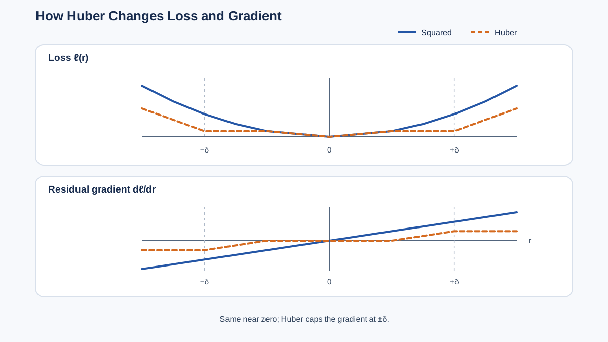
Huber loss keeps the quadratic penalty for small residuals and switches to a linear penalty once a residual crosses a threshold :
The two pieces meet at . Check the value: at , the quadratic piece gives , and the linear piece gives . Same number. Check the slope: the quadratic piece has slope at that point, and the linear piece has slope for all . Same slope. The loss is continuous and smooth at the changepoint, which is why gradient-based fitting behaves well.
Now differentiate:
Inside the quadratic region, the residual-gradient is the residual itself. Outside it, the residual-gradient is capped at magnitude . No matter how far a point drifts, its residual-gradient never exceeds .
That cap is the entire robustness story. Interpret as the boundary between "ordinary noise" and "large deviation." It is a modeling decision about what counts as an outlier, not a universal constant.
Two limits are worth memorizing. As , every residual falls in the quadratic region and Huber becomes squared error. As , the quadratic region shrinks to nothing and Huber approaches absolute error, whose residual-gradient is always . Huber lives between those two poles, and is the dial.
One property keeps Huber practical: it is convex. The piecewise definition looks like a kink, but the slopes match at the boundary, so the function curves smoothly and gradient descent still converges reliably.
From Residual-Gradient to Parameter Pull
Here is the bridge that keeps this from becoming a story about a single number. The residual-gradient is not the same thing as the gradient with respect to the model parameters. For a linear predictor , the chain rule gives
The parameter gradient for one example is the residual-gradient multiplied by the feature vector. Huber caps the first factor at ; it does not cap the second. A point with large feature values still contributes a larger parameter update than a point with small feature values, even when both sit in the linear region.
So the honest statement is narrower than "Huber caps a point's pull." Huber caps the loss-side factor. The feature values still scale the parameter contribution. If you want to reason about which points steer the fit, you need both pieces: how far the residual is, and how large the feature vector is.
Knowledge check
Check your understanding
Answer this question before you continue.
Worked Comparison: One Extreme Residual, Two Objectives
Numbers beat adjectives. Take five points with residuals of , , , , and one extreme point at . Fix .
| Residual | Squared error | Huber, | Squared residual-gradient | Huber residual-gradient |
|---|---|---|---|---|
| 0.5 | 0.5 | |||
| 0.125 | 0.125 | |||
| 0.125 | 0.125 | |||
| 0.5 | 0.5 | |||
| 50.0 | 9.5 |
The four ordinary points behave identically under both losses. The extreme point is where the objectives diverge. Squared error charges it 50; Huber charges it 9.5. More importantly, squared error assigns it a residual-gradient of 10, while Huber assigns it a residual-gradient of 1 — the same as a residual of 1.
Now double the extreme residual to :
| Residual | Squared error | Huber, | Squared residual-gradient | Huber residual-gradient |
|---|---|---|---|---|
| 200.0 | 19.5 |
Squared error's penalty quadrupled and its residual-gradient doubled. Huber's penalty roughly doubled and its residual-gradient did not move at all. The point can run to infinity and its loss-side factor stays pinned at . Its parameter contribution still scales with its features, but the residual no longer amplifies it.
You can reproduce and modify this in a few lines:
import numpy as np

def huber(delta, r):
    r = np.asarray(r, dtype=float)
    return np.where(np.abs(r) <= delta, 0.5 * r**2,
                    delta * (np.abs(r) - 0.5 * delta))

r = np.array([-1.0, 0.5, -0.5, 1.0, 10.0])
print("squared:", 0.5 * r**2)
print("huber:  ", huber(1.0, r))
Change delta to 0.5 or 5.0 and watch the extreme point's contribution move. That sensitivity is the next section.
Knowledge check
Check your understanding
Answer this question before you continue.
What Delta Actually Controls
is not a magic number. It is a residual-scale threshold that controls where the loss transitions from quadratic to linear. Moving it changes the fit's personality.
- Small : most residuals land in the linear region. The fit behaves closer to median-seeking, which can ignore large errors that are genuinely informative.
- Large : most residuals land in the quadratic region. The fit behaves almost like least squares, and the robustness you wanted largely disappears.
is also scale-dependent. A residual of 10 is extreme if your targets range from 0 to 20 and unremarkable if they range from 0 to 10,000. Set relative to the spread of the target, not as a fixed constant copied from a tutorial.
The practical consequence of a bad choice is symmetric. Too small, and you underfit real signal because the model treats legitimate variation as noise. Too large, and you inherit the exact outlier sensitivity you switched losses to avoid.
In practice, gets tuned alongside other hyperparameters on a validation set. The criterion is not "which makes the residuals look cleanest." The criterion is the evaluation metric or downstream cost you actually care about — validation RMSE, mean absolute error, or a business cost tied to specific error sizes. Pick the that wins on that metric, not the one that matches your intuition about which points are outliers.
Tip: Before tuning , plot the residuals from a squared-error fit. Large residuals clustering in a region you suspect is noisy is a reason to try Huber. Large residuals that look like real rare events are a reason to investigate the data, not to down-weight the points. Residual inspection is diagnosis, not proof.
Robust Is Not the Same as Correct
Here is the misconception worth killing: a robust loss does not fix unusual observations. It changes how much influence they have. Whether that influence should be reduced is a question about the data, not about the loss function.
If the extreme value is genuine and important — a real spike in demand, a real failure event — down-weighting it is a modeling error dressed up as robustness. You have told the model to ignore the thing you most needed it to learn.
Huber is also not immune to outliers. It still has a residual-gradient in the linear region; that gradient is just capped. Less sensitive is a different claim from insensitive, and the difference matters when many points sit in the tail.
It helps to see Huber as one option among several:
| Approach | Behavior on large residuals | When it fits |
|---|---|---|
| Squared error | Quadratic penalty, strong pull | Clean data; large errors genuinely worse |
| Absolute error | Linear penalty, constant pull | Median-seeking; heavy-tailed noise |
| Huber | Quadratic then linear at | You believe a subset of large residuals is noise |
| Target transform | Changes the error scale itself | Skewed targets; multiplicative error structure |
My rule is simple. Use squared error when large errors are genuinely worse and the data is clean. Consider Huber when you have a concrete reason to believe a subset of large residuals is noise. Investigate the points before choosing either.
One evaluation trap: a model trained with Huber can still be scored with RMSE. The training loss shapes the fit; the evaluation metric answers a separate question about the errors you care about. Do not assume they should match.
Where to Go Next
Before switching losses, inspect the residuals. Ask whether the large ones are noise or signal. That question determines the loss; the loss does not answer it for you.
Then run the experiment. Fit the same data twice — once with squared error, once with Huber — and plot the residuals for both. The places where the two fits disagree are the real output. Those disagreements tell you which points were steering the squared-error fit, and whether you wanted them to.
Knowledge check
Final check
Finish the article by checking the ideas you just learned.
References
Build stronger machine learning foundations
Use structured resources to connect theory, scikit-learn workflows, and evaluation practice.


