Outliers in Machine Learning: Remove Errors Without Deleting Rare Truth

Every beginner hits the same fork in the road. You plot your data, spot a few points sitting far from the pack, and freeze. Delete them? Keep them? The internet has strong opinions on both sides, and both sides sound convincing.

Here is the uncomfortable truth: outlier handling is not a yes/no decision. It is a classification task. Before you touch a single row, you need to answer two questions about each flagged value: Where did it come from? and What will it do to my model?

This guide walks through that decision process step by step, so you can handle extreme values with evidence instead of instinct.

Why Outliers Are Not One Problem

An outlier is simply a value that sits far enough from the rest of your data to raise suspicion about how it was produced. That distance is a symptom, not a diagnosis. The real question is what caused it.

Three common causes produce most outliers:

1. Measurement or entry errors. A sensor glitch, a typo, a decimal point in the wrong place. These values are noise, and they carry no useful signal.
2. Genuine rare events. A legitimate high-income customer in a spending dataset. A real system failure in a server log. These values are true observations, and they may matter enormously.
3. Heavy-tailed distributions. Some processes naturally produce extremes. Wealth, response times, and insurance claims all follow distributions where very large values are expected, not anomalous.

The same statistical distance can mean opposite things depending on context. A sensor reading of 500°C in a room-temperature dataset is almost certainly a broken instrument. A customer who spends 500 times the median in a retail dataset might be a fraudster, a business buyer, or your most valuable user. The number alone cannot tell you which.

This builds directly on the data preparation workflow you already know: inspect your raw rows, understand what each feature represents, and only then decide what needs cleaning.

How Outliers Actually Hurt Some Models

Here is the mechanism that matters: some models average, and some models rank. Averaging models feel outliers more.

Linear regression and other squared-error-based models minimize the mean squared error (MSE). Squaring errors gives large mistakes disproportionate weight. A single prediction that is off by 3 units contributes 9 units of squared error, while three predictions off by 1 unit each contribute only 3 units combined. One extreme value can pull the fitted line toward itself and inflate your error score, even when the model performs well on the other 99% of your data.

Tree-based models work differently. A decision tree splits on order rather than averaging distances. It asks "is this value above or below the threshold?" rather than "how far is this value from the center?" That makes trees naturally more resistant to extreme values. The same outlier that badly distorts a linear regression may barely change a decision tree trained on the same feature.

Your evaluation metric has the same sensitivity. Mean squared error amplifies outliers because squaring magnifies large errors. Mean absolute error (MAE) treats a loss of 3 as exactly three times worse than a loss of 1, not nine times worse. If you measure your model with MSE, a few extreme values can dominate your perceived performance.

Keep this mental handle: some models average, some models rank. Averaging models feel outliers more.

First, Inspect Before You Delete

Before choosing any response, you need to know what you are dealing with. Simple detection tools give you a starting point.

• Boxplots and IQR fences flag values beyond 1.5 times the interquartile range from the quartiles.
• Z-scores measure how many standard deviations a value sits from the mean.

Both tools have an honest limitation: they assume something about your distribution. Z-scores assume roughly normal data. IQR fences handle skew better but still misbehave on very skewed distributions, which are common in real tabular data. On a heavily skewed feature, these methods will flag legitimate tail values as outliers, sometimes by the hundreds.

A flagged value is a candidate for investigation, not a verdict. The threshold only tells you a value is unusual. It never tells you why.

So investigate. Look at the raw record. Check neighboring features for consistency. Ask whether the value is physically or logically possible. A temperature of 500°C is impossible in a room-temperature dataset. A purchase of 500 units might be a bulk order, a typo, or a data-entry artifact. The record itself often tells you which.

Plot the flagged point from two views: a boxplot shows you its rank, and a histogram shows you its context within the full distribution. Both views together tell a clearer story than either alone.

Four Defensible Responses, Not One Rule

Once you understand the cause, you have four defensible responses. Each matches a different diagnosis.

1. Keep and inspect

When the extreme value is a genuine rare event that carries real signal, removing it deletes information your model should learn. Fraud detection depends on rare fraudulent transactions. Anomaly detection in manufacturing depends on rare defect signatures. If your outlier represents a real phenomenon you care about predicting, keep it.

2. Transform

When a feature has a heavy-tailed distribution, a log or power transformation can compress extremes into a more modelable shape without discarding any data. This is often the right move for features like income, transaction amounts, or response times, where a few large values stretch the scale. The transformation changes the shape of the feature, not the meaning of the underlying measurement.

3. Use a robust model or metric

When extreme values are real but you do not want them to dominate, choose tools that resist them rather than altering your data. Tree-based models handle outliers gracefully. Absolute-error metrics like MAE stay honest when your data contains genuine extremes. This response keeps your data intact and changes the modeling approach instead.

4. Remove or correct

When the value is a confirmed measurement error or entry mistake, deleting or fixing it is defensible. A sensor that failed, a row where someone typed 500 instead of 50, a record with an impossible combination of values: these are not signal, and keeping them teaches your model noise.

The decision boundary maps cleanly: confirmed error means remove or correct. Genuine rare event means keep. Heavy-tailed distribution means transform or use robust tools. Real extreme that should not dominate means robust modeling.

The Leakage Trap in Outlier Handling

There is one trap that catches almost everyone at least once.

If you compute your outlier thresholds on the full dataset before splitting into training and test sets, you have just taught your model something about the test set. Your detection statistics were informed by values your model was never supposed to see. This is data leakage, and it inflates your apparent performance while hiding the truth about how your model will behave on new data.

The rule is simple: fit detection thresholds and transformation parameters on the training split only, then apply them to the test split. Any preprocessing decision informed by test data corrupts your evaluation.

This is exactly why outlier handling belongs inside a scikit-learn pipeline. A pipeline keeps your preprocessing steps bound to the training data, so the same transformation logic applies consistently at training and prediction time without leaking information across the split.

A Practical Decision Path for Your Data

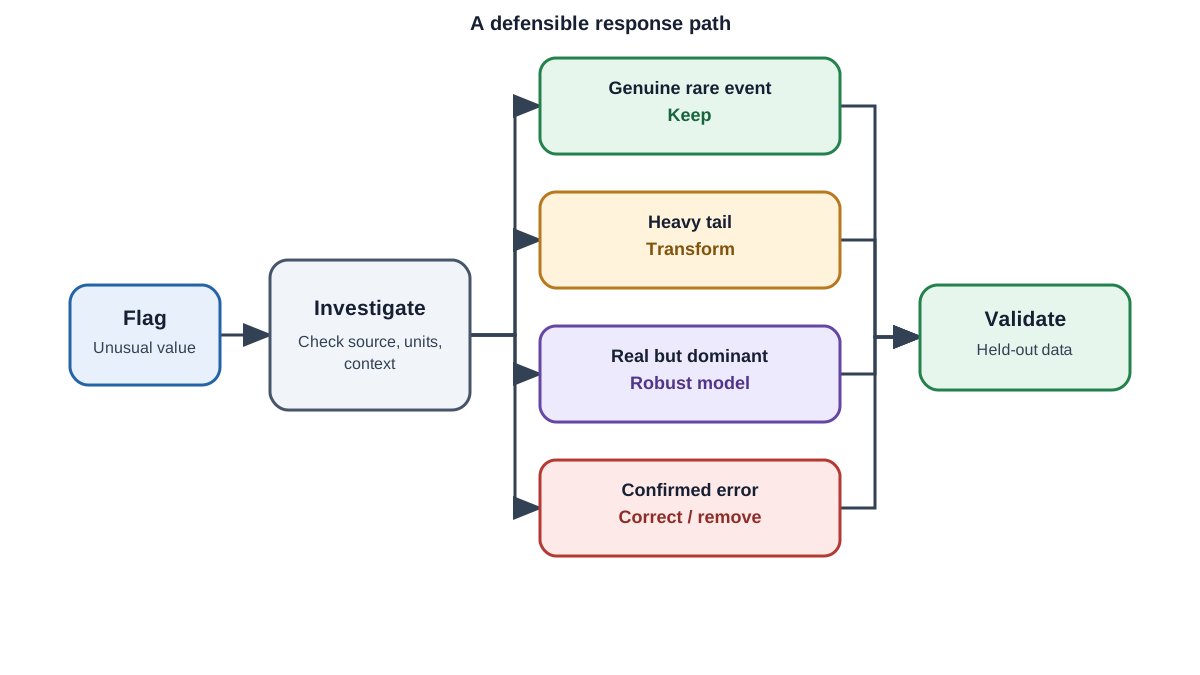
When you sit down with a new dataset, work through this sequence:

Step 1: Flag unusual values. Use a tool appropriate to your distribution. Boxplots and IQR fences for general exploration. Z-scores only when the data is roughly normal. Remember that flagged values are candidates, not verdicts.

Step 2: Classify each flagged value by cause. Is it a confirmed error? A genuine rare event? An expected tail of a heavy distribution? Look at the raw record. Check neighboring features. Ask whether the value is physically or logically possible.

Step 3: Choose the least destructive defensible response. Confirmed error means remove or correct. Real rare event means keep. Heavy tail means transform. Real extreme that should not dominate means robust modeling.

Step 4: Validate on held-out data. Compare model performance with and without your treatment. If removing a flagged value barely changes your results, you made a safe call. If it swings your metrics dramatically, investigate further before trusting either version.

The goal is a defensible, documented decision, not a perfect one. You should be able to explain why each extreme value was kept, transformed, or removed. That explanation is what separates thoughtful data preparation from arbitrary cleaning.

My rule after years of building models: the least destructive defensible option is usually the right starting point. Start by keeping your data intact. Transform when the shape demands it. Switch to robust models when extremes are real but dominant. Remove only when you have confirmed an error.

Outliers in machine learning are not a problem to eliminate. They are evidence to read. Some of that evidence is noise from a broken instrument. Some of it is the rarest and most valuable truth in your dataset. Your job is to tell the difference, and now you have a workflow that makes that judgment possible.

References

Research updated Sep 8, 2026