Polynomial Regression Explained: Make Curves With a Linear Model

You fit a straight line to data that clearly curves, and the line misses everything. Not by a little—systematically. It sits above the points in one region, below them in another, and no amount of tweaking the slope fixes it. The frustrating part is that the pattern isn't complicated. It bends once, maybe twice, and a simple curve would capture it beautifully.

Here's the counterintuitive fix: you don't need a new model. You need new features fed into the same linear regression you already know. That's polynomial regression in one sentence—and this article will show you why it works, where it breaks, and how to keep it honest.

When a Straight Line Just Won't Fit

Imagine you're modeling how a plant grows over a season. Early on, growth accelerates as the plant establishes itself. Then it slows, plateaus, and eventually levels off as resources run out. The relationship between time and height is real, smooth, and visibly curved.

Now fit a straight line through that data. The line has one slope, which means it can only move in one direction at a constant rate. It can't accelerate early and decelerate late. It cuts through the middle of the curve, missing the low points at the start, overshooting in the middle, and missing the plateau at the end.

The prediction equation for that line looks like what you already know:

ŷ = b₀ + b₁x

One intercept, one slope. The slope is a single number, and a single number cannot bend. That's the core limitation: a linear model with one feature draws a line, and a line has no curvature.

Here's the signal that a curve is hiding in your data: after fitting a straight line, plot the residuals—the differences between actual and predicted values. If the residuals show a pattern rather than random scatter—a smile, a frown, an S-shape—your line is missing structure. The pattern is the data telling you, in visual form, that the relationship bends.

The promise of polynomial regression is simple: keep the linear model, change the features, and get a curve.

The Trick: Add Powers of x as New Features

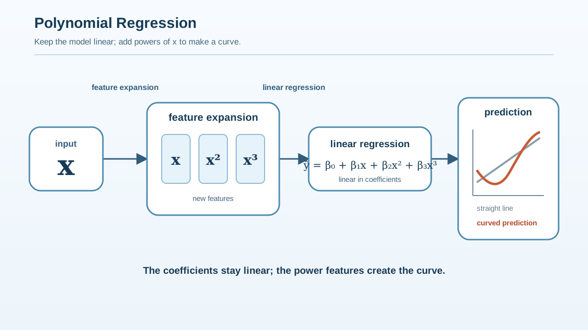
Here's the move that feels almost too simple: create a new column in your data that contains x², another with x³, and treat those columns exactly like any other feature.

This is feature engineering, not a new algorithm. You're not switching to a mysterious nonlinear method. You're giving your existing linear regression more columns to work with.

The expanded prediction equation for a quadratic model looks like this:

ŷ = b₀ + b₁x + b₂x²

Notice what changed. There's a new term, b₂x², but each term still has a single coefficient to learn. The model still computes a weighted sum of features. It still uses the same fitting procedure as ordinary linear regression.

This is the key distinction that confuses nearly every beginner: "linear" in linear regression refers to the parameters, not the shape of the curve. The model is linear because the prediction is a linear combination of the coefficients—each coefficient appears to the first power, multiplied by some feature. The features themselves can be x, x², x³, or anything else you can compute.

In scikit-learn, you create these features with PolynomialFeatures:

from sklearn.preprocessing import PolynomialFeatures

poly = PolynomialFeatures(degree=2, include_bias=False)
X_poly = poly.fit_transform(X)

The transformer takes your single feature column and produces new columns for x and x². Feed those into LinearRegression, and the model learns coefficients for both. The result is a curve.

To the model, x² isn't a mathematical operation. It's just another feature—a column of numbers with a coefficient attached. The math of linear regression never changes. Only the data does.

Note: This is why polynomial regression is sometimes described as a linear model for nonlinear relationships. The phrase sounds like a contradiction until you see that the linearity lives in the coefficients, while the curvature lives in the features.

Degree Controls Flexibility, Not a Fixed Number of Bends

The degree of the polynomial controls how flexible the curve can be:

• Degree 1: a straight line. The slope never changes.
• Degree 2: adds one curvature term, x². The curve can accelerate or decelerate once.
• Degree 3: adds x³, giving the slope another way to change direction.
• Degree 4 and up: more high-power terms, each permitting more complex shapes.

A common beginner mistake is to think degree 2 always produces one visible bend, degree 3 always produces two, and so on. That's not quite right. Degree sets the maximum complexity the curve can express, not a guarantee of how many turns it will use.

Think of it this way: a degree-3 model can produce a curve with two bends, but it might also settle on a shape that barely curves at all. Over your observed data range, a quadratic might look almost straight, and a cubic might show only one clear turn. The fitted coefficients decide what actually happens. What degree really buys you is room—more ways for the relationship between x and y to change as x moves.

Each increase in degree also adds new features. For a single input x, degree d produces features x¹, x², x³, up to xᵈ. With multiple inputs, the expansion includes interaction terms too. For two features at degree 2, you get x₁, x₂, x₁², x₁x₂, and x₂². The term x₁x₂ lets the effect of one input depend on the level of the other—a relationship a plain linear model simply cannot express.

Visualize the same dataset fit three ways. Degree 1 gives you a line that glides over the curve's shape, missing it systematically—underfitting. Degree 2 or 3 traces the curve smoothly, following the real pattern without chasing noise—a good fit. Degree 15 produces a curve that writhes through every training point, bending wildly to accommodate each individual observation—overfitting.

Here's a practical rule I've learned from building models: start with degree 2 or 3 and let validation tell you whether you need more. If your relationship needs degree 10 to look good on training data, you're probably fitting noise, not signal.

Why High Degree Means High Variance

When you raise the degree, you give the model more knobs to turn. Each new power of x is another coefficient the fitting procedure can adjust. More coefficients mean the model can contort itself to match the training data more precisely—including the parts of the data that are just random noise.

This is the bias-variance tradeoff showing up in concrete form. A low-degree polynomial has high bias: it's too simple to capture the curve, so it makes systematic errors. A high-degree polynomial has low bias on training data but high variance: it's so flexible that it memorizes the specific noise in your training set rather than learning the general pattern.

The practical symptom is unmistakable: great training error, poor performance on new data. The model performs beautifully on the points it has seen and falls apart on points it hasn't.

High-degree polynomials have another failure mode that catches people off guard: they behave erratically at the edges of the data range. Far from where any training points exist, the curve can shoot upward or downward dramatically. A degree-10 polynomial might fit your data beautifully between x = 0 and x = 10, then explode to absurd values at x = 11. The curve isn't just overfit—it's untrustworthy exactly where you might want to extrapolate.

Warning: Polynomial curves are global. A term added to fix a misfit in one region can push the curve around in another region far away. If your data has sharp local changes or you need reliable predictions beyond the observed range, a global polynomial is often the wrong tool.

Choosing the Degree With Validation, Not Vibes

So how do you pick the right degree? Not by staring at the training curve and admiring how well it hugs the points. Training error always improves as degree increases—that's the trap. The model gets more flexible, so of course it fits the training data better.

The principled approach is validation. Hold out a portion of your data, fit models at several degrees on the training portion, and evaluate each one on the held-out data.

The decision rule is simple: choose the degree where validation error stops improving. Watch the training-validation gap. As degree increases, training error keeps dropping. Validation error drops too—until it doesn't. At some point, validation error bottoms out and starts climbing back up while training error keeps falling. That widening gap is overfitting made visible. Pick the degree just before the gap starts to grow.

One workflow detail matters more than beginners expect: the polynomial expansion and any scaling must be learned inside the validation loop, not before it. If you expand features or scale them using the full dataset, information from your validation data leaks into the training process, and your error estimates become optimistically wrong.

The clean way to handle this in scikit-learn is a Pipeline:

from sklearn.pipeline import Pipeline
from sklearn.preprocessing import PolynomialFeatures, StandardScaler
from sklearn.linear_model import LinearRegression

model = Pipeline([
    ("poly", PolynomialFeatures(degree=3, include_bias=False)),
    ("scale", StandardScaler()),
    ("regress", LinearRegression())
])

The pipeline fits the polynomial expansion and the scaler only on the training fold each time, then applies those learned transformations to the validation fold. That keeps the whole procedure honest. Scaling matters here because polynomial features can span enormous ranges—if x goes from 1 to 10, then x¹⁰ is ten billion—and features at wildly different scales can cause numerical instability during fitting.

When Polynomial Regression Fits—and When It Doesn't

Polynomial regression is the right tool when you have a smooth, broad curve involving one or a few features, and you have reason to believe that relationship is polynomial-shaped. Domain knowledge helps here. Physical relationships often follow squared or cubed patterns—distance and gravity, area and scaling. Residual patterns from a linear fit also point the way: a clear curve in the residuals says a polynomial term might capture it.

It's also a sensible first step before reaching for more complex models. If a degree-2 or degree-3 polynomial handles your data well, you've solved the problem with a simple, interpretable model. No need to escalate to trees or other nonlinear methods.

But polynomial regression has real limits. With many features, the expansion explodes. Ten input features at degree 3 produce hundreds of terms, including all the cross-products. The model becomes hard to interpret, expensive to fit, and prone to overfitting. And because polynomial bases are global, they struggle with relationships that change character in different regions—sharp bends, local spikes, or plateaus that appear and disappear. When local behavior matters, splines give you more control by fitting piecewise curves that don't let one region's shape distort another's.

And when you want the flexibility of higher-degree terms without the runaway variance, regularization is the natural partner. Ridge or lasso regression penalize large coefficients, which keeps the curve from contorting wildly even when the degree is high. That combination—polynomial features plus regularization—is one of the most useful tools in classical machine learning.

The Next Experiment

Here's what I'd do next, and it takes ten minutes. Fit a linear model to your data. Plot the residuals. If you see a pattern, build a pipeline that creates polynomial features at degree 2 and degree 3, and compare cross-validated error against your degree-1 baseline.

Watch the training-validation gap as the degree climbs. That gap is the whole lesson of polynomial regression made visible: flexibility helps until it hurts. Find the degree where validation error stops improving, and you've found your curve.

References

Research updated Sep 8, 2026