Linear Regression From First Principles: Fit a Line, Read the Error

Most introductions to linear regression make it sound like drawing a line through some dots. That description is true and almost useless. Any line can be drawn. The real question is which line the data has earned—and how you know when the data has earned none at all.

Imagine you have a dataset of cars. For each car, you know its weight and its fuel efficiency in miles per gallon. Plot those points and you will see a pattern: heavier cars tend to drink more gas. The points scatter, but the trend leans downhill.

You want to predict fuel efficiency for a car you have not weighed yet. A straight line through that cloud of points would let you do it. But there are infinitely many lines you could draw. Some will slope too steeply. Some will sit too high. Some will chase a single outlier and ignore the crowd.

Linear regression is the discipline of choosing that line with evidence instead of intuition. It is the simplest supervised learning model in machine learning, and it is the right place to build your mental foundation.

What Linear Regression Actually Does

Linear regression predicts a continuous numeric target from one or more features. If you have read about regression versus classification, you already know the task: the target is a number like price, temperature, or fuel efficiency, not a category like "spam" or "not spam." Linear regression is one concrete model for that task.

The model itself is a straight line when you have one feature. Add a second feature and the model becomes a flat plane floating above the data. Add more features and the shape becomes harder to picture, but the logic stays the same.

What defines that line or plane is a set of parameters: an intercept and one coefficient for each feature. The intercept tells you where the line crosses the vertical axis. Each coefficient tells you how steeply the line rises or falls as that feature changes.

Fitting the model means choosing those parameters. Not by eyeballing the plot and sketching what looks right, but by letting a precise rule decide.

The Prediction Equation, Piece by Piece

Here is the equation for a model with one feature, written in plain language:

predicted value = intercept + (coefficient × feature value)

In symbols, that looks like:

ŷ = b + w₁x₁

The little hat on the ŷ is worth pausing on. It means "predicted." The actual fuel efficiency of a specific car is just y. The value our line produces is ŷ. The gap between those two is where all the interesting action happens.

Each symbol has a job:

• ŷ is the prediction the model makes.
• x₁ is the feature—in our example, the car's weight.
• w₁ is the coefficient, also called the slope or weight. It says how much the prediction changes when the feature increases by one unit.
• b is the intercept. It is the predicted value when the feature is zero.

Let us make that concrete. Suppose a fitted model for our cars produces this illustrative equation:

ŷ = 34 + (−4.6) × weight

The coefficient of −4.6 means that for every additional unit of weight, predicted fuel efficiency drops by 4.6 miles per gallon. The negative sign is the model saying: heavier cars use more fuel. The intercept of 34 is the predicted efficiency for a car weighing zero—which is nonsense in the real world, but the intercept still has a mechanical job to do. It anchors the line at a useful height.

Now predict for a car that weighs 4,000 pounds:

ŷ = 34 + (−4.6 × 4) = 34 − 18.4 = 15.6

The model predicts about 15.6 miles per gallon. That is the whole act of prediction: plug in a feature value, let the equation do arithmetic, read the answer.

When you have more than one feature, each one gets its own coefficient, and the predictions add together:

ŷ = b + w₁x₁ + w₂x₂ + w₃x₃

A car's efficiency might depend on weight, engine size, and number of cylinders. Each feature contributes its own push to the final prediction. This is called multiple linear regression, and it is the same idea wearing more clothes.

Why "Best" Means Least Squares

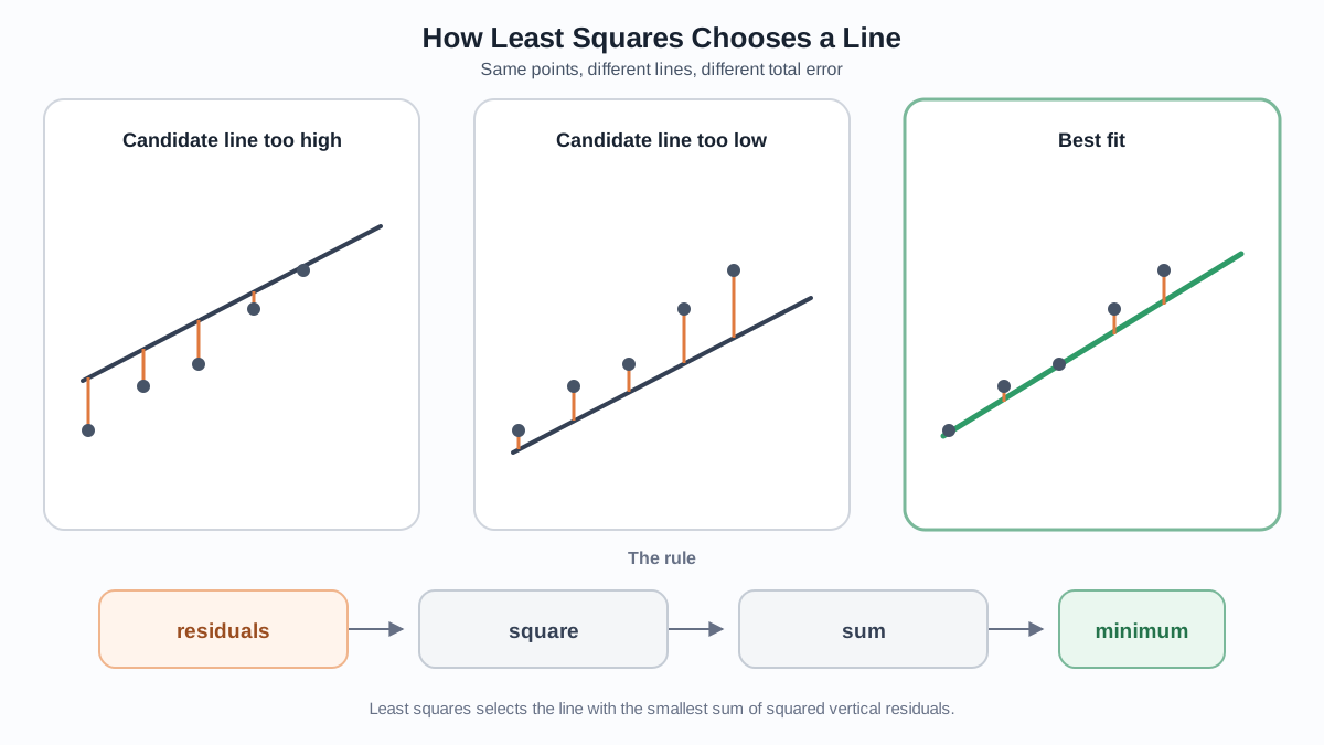
So we have a line. But which line?

Every candidate line makes mistakes. For each car in the dataset, the line produces a prediction, and that prediction differs from the actual observed efficiency. Those differences have a name: residuals. A residual is the vertical gap between a data point and the line—the part of reality the model failed to predict.

You might think the obvious goal is to make the residuals as small as possible. But there is a subtlety. Some residuals are positive (the line under-predicts) and some are negative (the line over-predicts). If you simply added them up, they would cancel each other out. A line that is wildly wrong in both directions could look perfect.

Squaring the residuals solves that problem. A squared residual is always positive, whether the original error was +5 or −5. Squaring also punishes big misses more than small ones. Missing by 10 units costs four times as much as missing by 5, not twice as much. That is a deliberate choice: large errors are usually worse than small ones, and the squared penalty reflects that judgment.

The rule that chooses the line is therefore called least squares. Among all possible lines, pick the one that minimizes the sum of the squared residuals. That line is the best-fitting straight line in a precise, mathematical sense.

This objective should feel familiar if you have seen regression evaluation before. The mean squared error, or MSE, is just this same sum averaged over the number of data points. Fitting a linear regression model and evaluating it are two sides of the same coin: the model is trained to minimize exactly what you later measure.

Reading the Coefficients and the Residuals

Once the model has found its line, the real work begins: interpretation.

A coefficient is a claim about the relationship between a feature and the target. A coefficient of −4.6 says the relationship is negative: as weight goes up, efficiency goes down. A coefficient of +3 would say the opposite. The sign tells you direction. The magnitude tells you strength—how much the target moves for each one-unit change in the feature.

There is a crucial qualifier when you have multiple features. Each coefficient describes the change in the target per one-unit change in that feature, holding all other features fixed. This is not a small technicality. If you include both weight and engine size in a model, the coefficient on weight is not "what happens when weight changes in the real world." It is "what the model predicts when weight changes and engine size stays the same." Real cars do not work that way, which is why you must read coefficients as conditional claims, not universal truths.

The residuals deserve just as much attention as the coefficients. After fitting, every data point has a leftover error. Small residuals mean the line captures most of the pattern. Large residuals mean the model is missing something.

Here is the mental shift that separates people who understand regression from people who just run it: residuals are not noise to ignore. They are evidence.

Plot the residuals against the feature values. If the plot looks like a random cloud, the straight line has captured the pattern you can see. If you see a curve—residuals that dip down at the left, rise in the middle, and dip again on the right—the model has missed a bend in the data. If the residuals fan out like a trumpet as the feature grows, the model's errors get worse as values get larger. Both patterns are the data telling you that a straight line is the wrong shape.

Note: A patternless residual plot is good evidence that no obvious shape remains. It is not proof that the model is trustworthy. A line can still mislead if you predict far outside the range of your data, if a few unusual points are pulling the fit, or if the model performs poorly on data it has not seen. Residuals tell you what shape the model missed. They do not tell you everything about whether the model will travel well.

What "Assumptions" Really Mean

You will hear that linear regression has assumptions. That word sounds like a checklist you must memorize. Think of it differently: assumptions are the conditions under which the fitted line, its coefficients, and its uncertainty estimates can be trusted.

For a beginner, three conditions matter most.

The relationship should be roughly linear. If the true pattern is curved, a straight line will miss it in a systematic way. This is the assumption that most directly affects prediction quality.

The residuals should have a sensible spread. If the errors fan out or tighten as the feature grows, the model is not equally reliable across the data. This matters for understanding where your predictions are trustworthy.

The observations should be independent. If your data has a natural order or grouping—time series, repeated measurements from the same car—the errors may influence each other. That hidden dependence can make your model look more reliable than it is.

There is a fourth condition you will see in many textbooks: the residuals should be roughly bell-shaped. For basic prediction, this matters less. It becomes important when you want formal confidence intervals and significance tests, which rely on that shape. A beginner can set that concern aside until the need for statistical inference arrives.

The practical rule is simpler than the checklist. Fit the line. Plot the residuals. Ask whether the pattern looks straight, whether the spread looks even, and whether your data has hidden structure that a straight line cannot honor.

When a Straight Line Helps, and When It Lies

Linear regression is a tool with a clear boundary. Inside that boundary, it is remarkably useful. Outside it, it will produce confident nonsense.

The model shines when the relationship between features and target is roughly straight and you want a simple, interpretable model. That combination is more common than you might think. Many relationships in real data are approximately linear over the range you care about. And the model's transparency is a genuine asset: you can read the equation and explain to someone else exactly what the model believes.

The model fails in recognizable ways. If the true relationship is curved, no straight line will capture it. If a single outlier sits far from the rest of the data, least squares will drag the line toward it, because squaring that one huge error makes it very expensive to ignore. If your features are strongly correlated with each other, the individual coefficients become unstable and hard to trust.

The linearity assumption is the first thing to check. A scatter plot of the data, or a plot of residuals after fitting, will reveal curvature that a straight line cannot represent. This is not an advanced diagnostic. It is the basic due diligence of using the model at all.

Common mistake: Assuming that because a line fits, the relationship is truly linear. A straight line can always be drawn through any cloud of points. Whether that line means something is a separate question—one the residuals help you answer.

Even when a straight line is not the final answer, it still has value as a baseline. A simple linear model gives you a reference point. If a more flexible model cannot beat it meaningfully, the extra complexity may not be worth carrying.

Your First Experiment

Here is where to start: take a small dataset with one feature and one numeric target. Fit a straight line. Then look at the residuals.

Do not rush to evaluation metrics. Do not reach for a more complex model. Just fit the line, plot the residuals, and ask two questions. Are the residuals small relative to the scale of the target? And do they show any pattern, or do they look like random scatter?

Then use what you see:

• Random scatter with small residuals: The line is a reasonable baseline. Keep it.
• A clear curve: The model missed a bend. A nonlinear pattern or an additional feature may be needed.
• A fan shape: The errors grow with the feature. The model is less reliable at the wide end.
• A few extreme residuals: Look at those points. They may be unusual observations worth investigating, not just errors to delete.

That single habit—fit a line, then read the error—will teach you more about regression than any amount of abstract study. It will also build the instinct you need for every model you learn afterward. Linear regression is the first straight-line claim you will make about data. Learning to hear what the residuals say is how you will know whether that claim holds.

References

Research updated Sep 8, 2026