Generalized Linear Models Explained: Extend Linear Thinking Beyond Straight Lines

Linear regression draws a straight line through continuous numbers. Logistic regression draws an S-curve that outputs probabilities. They look like completely different tools—different math, different loss functions, different mental pictures. So you file them away as separate recipes and move on.

Here is the reframe that saves you from that fragmented mental model: they are the same engine wearing different output layers. The engine is a weighted sum of your features. What changes is what you do with that sum before it becomes a prediction. Generalized linear models explained in one sentence: keep the linear core, swap the output machinery to match the kind of outcome you are predicting.

Why Linear Regression and Logistic Regression Feel Like Different Tools

The surface difference is real. Linear regression predicts a continuous value directly—house prices, temperatures, test scores. Logistic regression predicts a probability that must stay between 0 and 1—will this customer churn, does this email look like spam, is this tumor malignant?

But look under the hood and you will find the same engine running in both cases: a weighted sum of features. In linear regression, you compute that sum and call it the prediction. In logistic regression, you compute that sum and then push it through a transformation that squeezes it into the 0-to-1 range before calling it a probability.

The GLM framing makes this explicit. The weighted sum is the engine. The difference between models is what happens to that sum before it becomes a prediction. Once you see that, logistic regression stops being a separate algorithm and becomes a special case of a broader family—one that also includes models for count data, rates, and other outcome types you cannot reasonably fit with a straight line.

The Three Pieces of Every Generalized Linear Model

Every generalized linear model has three structural pieces. Once you name them, the whole family stops being a grab bag of unrelated techniques.

Piece one: the linear predictor. This is the familiar weighted sum from linear regression. Each feature gets a coefficient, you multiply and add, and out comes a single score. Nothing new here—you already know this equation.

Piece two: the link function. This is the bridge that maps the linear predictor onto the scale where your outcome actually lives. The link function is what lets one linear engine handle very different kinds of targets.

Piece three: the response distribution. This is your assumption about what kind of outcome you are modeling—continuous, binary, count—and how the noise around your predictions behaves.

Think of it this way: the linear predictor is the engine, the link function is the transmission, and the response distribution is the road surface the model must drive on. The engine stays the same. The transmission adapts its power to the terrain. And the road surface determines what kind of driving is even possible.

Link Functions: The Bridge Between a Score and an Outcome

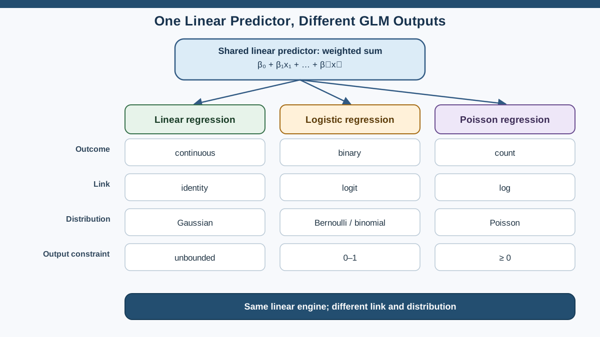
The link function is where the real magic happens, so let us look at three common ones.

The identity link does nothing. The linear predictor passes straight through to become the prediction. This recovers ordinary linear regression for continuous outcomes. If your outcome is roughly symmetric, unbounded, and continuous, you do not need a bridge at all.

The logit link is what logistic regression uses. It takes a linear score that could be any real number—negative, positive, huge—and maps it into a probability between 0 and 1. That S-curve you have seen is not a sign that the model went nonlinear. The model is still linear in its parameters. The link function is simply bending the output to respect the fact that probabilities cannot go below 0 or above 1.

The log link keeps predictions positive, which makes it the natural choice for count data. Number of purchases, number of clicks, number of insurance claims—these cannot go below zero, and a linear predictor that outputs −3 is meaningless for them. The log link ensures the model only produces non-negative predictions.

Here is the key insight: the link function is chosen to match the outcome's natural constraints, not for cosmetic reasons. This is also where beginners get confused. They see the S-curve of logistic regression and assume the model is nonlinear. It is not. The model is still linear in its parameters—the coefficients still add up in a straight line. Only the link bends the output.

Common mistake: Calling a GLM "nonlinear" because the output curve bends. The model is linear in its parameters. The link function is what bends the output to respect the outcome's constraints.

Response Distributions: Matching the Model to the Data's Shape

The response distribution is the third piece, and it matters more than most introductions let on. It is not a formality. It changes how the model treats errors and what predictions it considers plausible.

Ordinary least squares assumes a normal (Gaussian) distribution around the mean. That assumption suits symmetric continuous noise—measurement error, natural variation around an average. When your outcome is roughly bell-shaped around the prediction, this is the right tool.

Binary outcomes call for a binomial or Bernoulli distribution. This is why logistic regression treats each prediction as a probability rather than a raw score. The distribution knows the outcome can only be 0 or 1, and it shapes the model's behavior accordingly.

Count data—number of events, purchases, clicks, claims—fits a Poisson distribution. The Poisson keeps predictions non-negative and, crucially, handles the fact that variance grows with the mean. Count data does not have constant spread. Days with more traffic also have more variable traffic. A normal distribution cannot capture that; a Poisson can.

The distribution choice changes how the model weights errors. If you fit a normal distribution to count data, the model treats a prediction of 50 with an observed value of 100 as a moderate miss. A Poisson-based model understands that when the mean is 50, seeing 100 is far more surprising—and weights that error accordingly.

In scikit-learn, this family is available through PoissonRegressor, GammaRegressor, and TweedieRegressor, which sit alongside LinearRegression in the linear model module.

When a GLM Beats Ordinary Least Squares

Here is the decision rule I use: ask what the outcome can and cannot be, then pick the distribution and link that respect those constraints.

Use a GLM when the outcome is bounded, discrete, or skewed in a way a normal distribution cannot capture. The failure modes of forcing ordinary least squares onto such data are concrete and easy to spot.

Fit OLS to a binary outcome and you will get predictions below 0 or above 1. Those are meaningless as probabilities, yet the model will happily produce them. Fit OLS to count data and you will get negative predictions for things that cannot be negative—negative purchases, negative clicks—while also ignoring that the variance grows with the mean.

When is ordinary least squares still fine? When your outcome is continuous, roughly symmetric, and has no hard bounds. Temperature, height, test scores, profit margins—these fit the normal assumption well enough that a GLM adds complexity without adding much.

Note: The GLM framing is not about being fancy. It is about refusing to force data into a shape it does not have. Name the outcome's constraints first. Then choose the model that respects them.

Where the GLM Framework Stops Being Enough

Every framework has a boundary, and the GLM's is worth naming clearly.

A GLM is still linear in its parameters. It cannot learn feature interactions on its own, and it cannot model genuinely nonlinear feature effects. If the relationship between a feature and the outcome is curved—say, age and risk follow a U-shape—a GLM will miss it unless you manually add polynomial terms or interaction features.

The GLM's strength is interpretability and a principled match to the outcome type, not raw predictive flexibility. You get coefficients you can read and explain. You get a defensible statistical foundation. You do not get automatic discovery of complex patterns.

When the relationship between features and outcome is genuinely curved or interactive, tree-based models or other flexible approaches will often fit better. That is not a dismissal of GLMs. It is an honest boundary.

My rule: reach for a GLM when you want coefficients you can read, a principled match to the outcome type, and a strong baseline before trying more complex models. In many real projects, that baseline is good enough to ship.

The Practical Takeaway

Before you fit any model, name the outcome's constraints. Is it continuous and unbounded? Binary? A count that cannot go negative? Skewed so that variance grows with the mean?

Then choose the distribution and link that respect those constraints. Continuous and symmetric? Ordinary least squares. Binary? Logistic regression with a logit link. Count data? Poisson regression with a log link.

The GLM framework is not another algorithm to memorize. It is the connective tissue that shows you why these models exist and when each one earns its place. The engine is always the same linear predictor. The link function and response distribution are how you adapt that engine to the reality of your data.

Try it on your own data. Take a binary or count outcome you have been forcing through ordinary least squares, reframe it as a GLM, and watch what changes. The predictions will respect the outcome's constraints. The coefficients will still be readable. And the mental model you build from that exercise will serve you across every linear model you touch afterward.

References

Research updated Sep 8, 2026