
How Neural Networks Build Representations Through Layers
You have already done the thing this article is about. You looked at a column of raw numbers, decided that a ratio or a logarithm would be more useful,…

Key topics
You have already done the thing this article is about. You looked at a column of raw numbers, decided that a ratio or a logarithm would be more useful, created that column by hand, and watched your model improve. Then you asked the question that starts every serious machine learning conversation: who decides which features matter?
A neural network answers that question by learning the transformation itself. Not magic. Not a black box that "just figures it out." A stack of small, learnable transformations, each one rewriting the data before the next one reads it.
If you have already worked through the data–objective–training loop and the classical-versus-deep-learning decision, you have the background you need. This article stays on the mechanism: what a unit computes, why stacking units changes what a model can represent, and where the analogy to classical feature engineering stops being useful.
The Feature You Used to Write by Hand
Recall the classical workflow. You inspect the data, notice that a ratio between two columns might separate the classes better than either column alone, and you write that ratio into a new column. You might add a log transform to tame a skewed distribution, or a squared term to let a linear model bend. Then you hand the whole table to scikit-learn and let it fit weights on top.
Here is the part worth sitting with: the representation is frozen before training starts. The model learns how much to trust each column you gave it. It does not learn what the columns should be.
That is not a flaw. It is a design choice, and it is often the right one — hand-designed features encode real domain knowledge, and on small tabular problems they frequently beat anything a network learns from scratch. But it does set a ceiling. If the pattern you need lives in a combination of inputs you did not think to write down, no amount of optimizer effort will find it. The model can only reweight the world you handed it.
So the central question becomes concrete: what changes when the transformation from raw inputs to useful intermediate values is learned during training, instead of written by hand beforehand?
Knowledge check
Check your understanding
Answer this question before you continue.
One Unit: A Weighted Sum With a Switch
Start with the smallest object in the whole story. A single unit — often called a neuron — takes several numbers in, multiplies each by a weight, adds the results, adds one more number called a bias, and then passes that total through an activation function.
In one expression:
output = activation( w₁x₁ + w₂x₂ + ... + wₙxₙ + b )
Each symbol does one job. The inputs x are the numbers arriving from the previous stage. The weights w say how much each input matters to this unit. The bias b shifts the total up or down, the way an intercept shifts a regression line. The activation is the switch.
Plain English: a unit is a tiny linear model with a nonlinear gate bolted to its output. The weighted sum is the linear part — the same arithmetic as logistic regression. The activation is what makes it something more.
Why does the gate matter so much? Because without it, stacking units accomplishes nothing. A weighted sum of weighted sums is still a weighted sum. Chain ten linear transformations together and you get one linear transformation wearing a costume. The nonlinearity is the entire reason depth is worth anything.
Note: Common activation functions include sigmoid, tanh, and ReLU. You do not need to pick one yet. What matters is that the function is nonlinear, so the unit's output is not a straight-line function of its inputs.
Knowledge check
Check your understanding
Answer this question before you continue.
A Layer Is Many Units Reading the Same Input
A layer is not a new kind of object. It is many copies of the unit you just learned, all reading the same input vector at the same time, each producing its own output number. Collect those outputs and you have a new vector — the layer's output.
That parallel structure is where specialization begins. One unit might learn to respond strongly when two particular inputs are both large. Another might respond to a completely different combination. Neither unit knows what the others are doing; they simply produce their numbers, and the next stage decides what to do with them.
Then comes the trick that makes the whole architecture work: the output vector of one layer becomes the input vector of the next. The second layer does not see your original columns. It sees the first layer's outputs. It applies its own weighted sums and switches to those numbers.
A layer that talks only to other layers — not to the raw input, not to the final answer — is called a hidden layer. The name is less mysterious than it sounds. It is hidden because you never observe its values directly in your dataset; they are computed fresh for every input.
Tip: Picture two stacked layers with the intermediate vector drawn between them. Label that middle vector "the representation." That label is the whole idea of this article in one word.
Knowledge check
Check your understanding
Answer this question before you continue.
Depth as a Chain of Rewrites
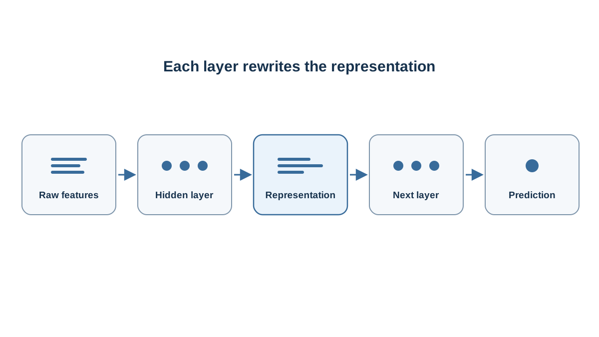
Here is the mental model I want you to keep.
Each layer is a translator. It takes the data as written in the previous layer's language and rewrites it into a new language. The next layer never reads the original text — it only reads the translation. By the time you reach the final layer, the data has been rewritten several times, and each rewrite was shaped by training to make the final answer easier to produce.
Early layers tend to encode simple combinations of the raw inputs. Later layers combine those into more abstract ones. The final layer is usually a plain linear model — a weighted sum with no switch, or a softmax for classification. All that depth exists to build a representation that a simple final model can separate.
Now compare that to your scikit-learn pipeline. There, you fix the transformation, then fit the model. Two separate steps, two separate decisions. Here, the transformation and the model are fit together, by the same objective, at the same time. The feature engineering is not a preprocessing stage. It is part of the model.
Common mistake: Assuming each hidden unit has a clean, nameable meaning like "this unit detects edges" or "this unit detects price sensitivity." Sometimes a unit correlates with something interpretable. Often it does not. The representation is distributed across many units, and the metaphor of translation is a guide, not a promise.
Watching a Representation Change
Abstractions like "the layer rewrites the data" stay slippery until you trace one small case. So let us trace one.
Imagine two input features, x₁ and x₂, and a pattern that is hard to separate in the raw space: the positive class sits near the diagonal where x₁ and x₂ are both large or both small, and the negative class sits where one is large and the other is small. A straight line through the original two features cannot cleanly divide those groups.
Now suppose the first layer contains two units, and training settles on weights that make one unit respond mostly to x₁ + x₂ and the other respond mostly to x₁ − x₂. Those are not exotic operations — they are just weighted sums with weights of (1, 1) and (1, −1). But look at what they do to the data. In the new two-number representation, the diagonal pattern from the original space becomes a simple split along one axis. The positive class clusters at high values of the first new number; the negative class clusters at low values. A final linear layer can now separate them with a single threshold.
Nothing about the original problem changed. The data was rewritten into a space where the pattern is easier to see. That is the whole mechanism of depth in one example: each layer hands the next layer a representation in which the remaining problem is simpler.
You have met this idea before. Kernel methods and polynomial feature expansion exist for exactly this reason: they transform the inputs so a linear model can draw a boundary that was impossible before. The difference is who chooses the transformation. With a polynomial expansion, you decide the degree. With a kernel, you pick the kernel. With a neural network, the transformation is learned from data.
That is the real claim behind "neural networks learn their own features." They can encode combinations you did not think to write down, because the combinations are parameters, not decisions.
Why This Beats Fixed Features on Some Problems
The advantage is easiest to see on a pattern that is not linearly separable in the original inputs but becomes separable after a nonlinear rewrite — exactly the case we just traced.
But this is a tradeoff, not a free upgrade. More parameters mean more data needed to fit them, and less interpretability of any individual feature. A coefficient in a linear model tells you the direction and size of one effect. A weight buried in the third hidden layer of a network tells you almost nothing on its own.
| Situation | Sensible starting point |
|---|---|
| Small tabular dataset, good hand-built features | Gradient-boosted trees or regularized linear models |
| High-dimensional input, plenty of data | Learned representations become worth the cost |
| Pattern not linearly separable in raw inputs | Either an explicit feature expansion or a learned one |
The honest summary: on a small table where your engineered features already separate the classes, a boosted tree will often win, and it will be faster to train and easier to explain. Reach for learned representations when the input is high-dimensional and you have enough data to fit many parameters without memorizing noise.
What Training Is Actually Adjusting
Every weight and every bias in every layer is a parameter. The intermediate activations — the numbers flowing between layers — are not stored knowledge. They are recomputed from scratch for each input.
Training works like this. A loss function scores the final output against the target. That score produces an error signal, which is propagated backward through the network to update every layer's weights — including the early layers that produced the representation. The same gradient signal that adjusts the output layer also adjusts the translators underneath it.
This is the sharpest difference from a scikit-learn pipeline. There, the feature transform has no fitting step of its own; it is fixed before the model sees data. Here, the transform is updated by the same signal as the output layer, which is why the representation and the prediction improve together.
I am deliberately not re-deriving the update mechanics here. The gradient descent and loss function articles cover how a loss guides parameter updates and how different loss choices change behavior. What matters for this mental model is the consequence: because early layers are updated by a signal that traveled through many layers, training depth is genuinely harder than training a single linear model. That difficulty is not a bug in your code. It is the nature of the problem.
Knowledge check
Check your understanding
Answer this question before you continue.
Where the Mental Model Breaks Down
A good mental model gets you started. Knowing its edges keeps it from fooling you.
More layers do not automatically mean better representations. Depth without enough data, enough signal, or enough care tends to overfit. The network memorizes the training set and generalizes poorly.
Individual units are usually not clean, nameable features. The interpretability you get from a linear model's coefficients does not transfer. If you expect every hidden unit to have a tidy meaning, you will be disappointed — and that disappointment is normal, not a sign you misunderstood.
The model has no notion of which inputs are meaningful. It will happily learn from noise if the data lets it. Feature quality still matters; it just enters the system differently.
A basic feed-forward network treats each example as a fixed input-to-output mapping. It does not explicitly preserve sequence order or spatial structure. You can still feed it a fixed-size summary of sequential or image data, and it may work fine. But when that structure matters, architectures designed to use it — recurrent or convolutional models, for example — tend to be a better fit. This article stops at the mechanism and does not cover training tricks, regularization, or framework APIs.
What to Do With This Model Next
Keep one sentence: a neural network is a stack of learned feature transformations, where each layer rewrites the data into a new representation that the next layer reads.
Here is the decision rule. If your tabular problem is small and your engineered features already separate the classes, stay with classical models. Reach for learned representations when you have high-dimensional inputs and enough data to fit many parameters.
And here is the concrete next step. Take a dataset you have already modeled with logistic regression. Write down every feature interaction you had to build by hand — the ratios, the products, the squared terms. That list is exactly the kind of transformation a hidden layer would try to learn on its own. You do not need a framework to do this exercise. You just need to notice how much of your modeling effort went into deciding what the features should be, and how much went into fitting weights on top of them.
That ratio is the whole argument for representation learning, and now you can see the mechanism behind it.
Knowledge check
Final check
Finish the article by checking the ideas you just learned.
References
Build stronger machine learning foundations
Use structured resources to connect theory, scikit-learn workflows, and evaluation practice.


