Gradient Descent Explained: How Models Improve One Step at a Time

A model starts with random parameters and ends up making sharp predictions. Nobody tells it the answer. It just keeps nudging itself in the right direction until the errors shrink.

Here is the mental model that makes sense of it: training is a guided walk downhill. The loss function builds the terrain. The gradient points uphill—so you step against it. The learning rate sets your stride. Get those pieces straight, and gradient descent stops feeling like magic and starts feeling like the simple loop it really is.

The Puzzle: How Does a Model Get Better Without Being Told the Answer?

A quick recap of where we are. A model has parameters—numbers that shape its predictions. A loss function measures how wrong those predictions are. Lower loss means a better model. That part is probably familiar from earlier work with linear regression.

Here is the puzzle that follows: given a loss value, how does the model decide which way to nudge its parameters?

It cannot try every possible setting. There are too many. It cannot guess randomly and hope. That would take forever. And it certainly does not secretly know the right answer—if it did, training would be pointless.

So what does it do?

The answer is that the model reads the shape of its own errors. It looks at the current spot on a landscape built from the loss function, figures out which way is downhill, and takes a step. Then it looks again. Then it steps again. Repeat until the ground levels out.

That loop is gradient descent, and it is the engine behind much of machine learning. Once you see it clearly, you will recognize it everywhere.

The Loss Landscape: Turning Error Into a Terrain You Can Walk On

Here is the trick that makes optimization visual: for any set of parameter values, the loss function returns exactly one number—the total error. That means we can imagine every possible parameter setting as a position on a map, with the error as the elevation at that spot.

Picture a hilly terrain. Your horizontal position represents the parameter values. The height of the ground represents the loss. A high ridge means bad predictions. A valley means good ones.

Your goal is to find the lowest valley you can reach. Not necessarily to hit zero error—real data is noisy, and perfect predictions are usually neither possible nor desirable. You just want the lowest point available.

With one parameter, this landscape is a simple curve you can draw on paper. With two parameters, it becomes a bowl or a surface you could hold in your hands. With dozens or thousands of parameters—which happens in real models—the landscape exists in a space you cannot picture. But the logic does not change. You are still looking for the lowest point, and you still find it by walking downhill.

The loss function builds this terrain. Your job during training is to walk it well.

The Gradient: Read Uphill, Step Opposite

So you are standing somewhere on this loss landscape, and you need to know which way is down. That is exactly what the gradient tells you.

The gradient is a measure of the local slope. At your current position, it points in the direction where the loss surface rises most steeply. In plain language: the gradient tells you which way is uphill. So to reduce loss, you move in the opposite direction.

That is the whole idea behind gradient descent in one sentence: read uphill, step opposite.

Where does the gradient come from? It is computed from the loss function and your current parameters. It is not guessed and it is not random. Mathematically, it comes from derivatives—the calculus tool that measures how fast a function changes at a particular point. But you do not need to compute derivatives by hand to understand what is happening. Think of the gradient as a directional slope reading. It answers one question: if I nudge my parameters a little, which way makes the loss go down fastest?

One crucial detail: the gradient is local. It only describes the slope at the exact spot where you are standing. The terrain a few steps away might slope differently. That is why the model cannot just read the gradient once and be done. It has to take a step, re-read the slope, and take another step. Every update is based on fresh information about the current position.

The Update Rule: One Step at a Time

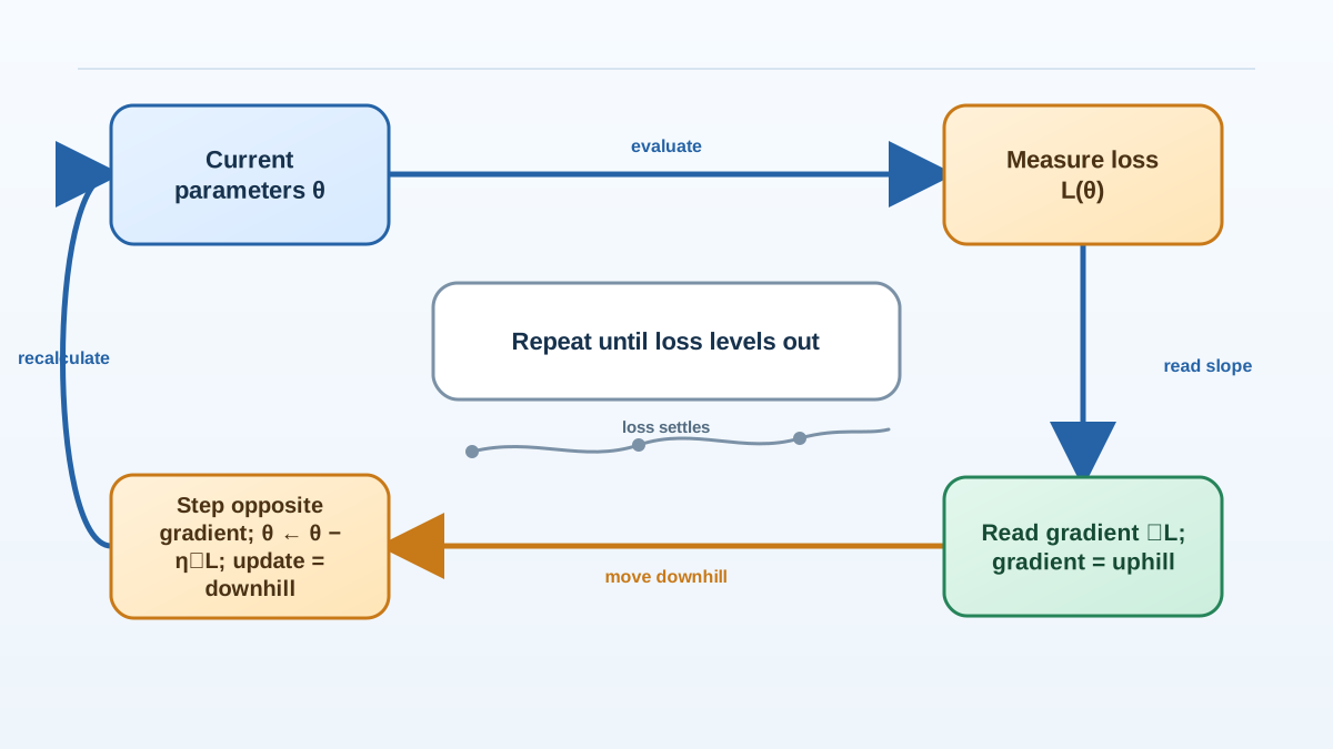
Now we can write the core loop of gradient descent. It is almost embarrassingly simple:

1. Calculate the loss with your current parameters.
2. Find the gradient—the direction that points uphill.
3. Move your parameters a small amount in the opposite direction.
4. Repeat.

Each repetition is called an iteration. The movement itself follows a pattern you will see everywhere in machine learning:

New parameter = old parameter − (learning rate × gradient)

Let us unpack that. The gradient gives you the direction. The learning rate gives you the step size. Multiply them together, subtract from where you are, and you have taken one downhill step.

Here is what that looks like with a single weight in a simple linear model. Suppose your current weight is 0 and your loss is about 300. The gradient at that spot is steep—say, roughly 60—and your learning rate is 0.02. Your update becomes:

New weight = 0 − (0.02 × 60) = −1.2

Wait—the weight moved to −1.2, not +1.2. The sign depends on how the loss changes as the weight increases. If the loss rises when the weight increases, the gradient is positive, and you subtract to move downhill. If the loss falls when the weight increases, the gradient is negative, and subtracting a negative moves you uphill in weight space—which is downhill in loss space. Either way, the rule is the same: step against the gradient.

After that first update, the loss drops to roughly 170. Another step brings the weight to about 2 and the loss to around 100. Another: weight near 2.7, loss near 69. Each step shrinks the error, but notice something important—the improvements get smaller as you go. The slope flattens as you near the bottom of the valley.

Eventually, further steps barely reduce the loss at all. That point is called convergence. The model has found parameters that produce nearly the lowest loss available on this terrain, and additional iterations are not buying meaningful improvement.

This is the moment training stops. Not because the model is perfect, but because it has reached the bottom of the valley it was walking toward.

Note: An iteration is one parameter update. The data used for that update is called a batch. When an implementation processes your entire dataset in one batch, a full pass through the data is called an epoch. Some algorithms update after every single example, some after small groups, and some only after seeing everything. The loop is the same; only the batch size changes.

The Learning Rate: Why Step Size Is the Knob That Matters Most

The learning rate is the hyperparameter that controls how far each step moves. For a beginner troubleshooting a model that will not train, it is often the first knob to check—because it determines whether your downhill walk ends in the valley or somewhere embarrassing.

Set the learning rate too large, and you overshoot. Imagine taking enormous strides down a hill—you blow past the valley floor and start climbing the opposite slope. The loss bounces around instead of settling. In the worst case, each step makes things worse, and the model diverges entirely. The loss grows instead of shrinking, and training is ruined.

Set the learning rate too small, and you creep. Every step is so tiny that reaching the bottom takes thousands of iterations. The model eventually gets there, but you waste enormous time watching it crawl. Small steps are safe, but they are slow.

Set it just right, and you get steady progress: large enough to move efficiently across flat regions, small enough to avoid skipping past the minimum when the terrain curves.

Here is the decision rule I use when something goes wrong: if your loss is bouncing around or growing, your step is probably too big. If training crawls and barely improves, your step is probably too small. The loss curve tells you which failure mode you are in.

In practice, the learning rate is rarely a single fixed number. Many training routines start with a larger rate and shrink it over time, letting the model move quickly early on and settle gently near the end. Scikit-learn and other libraries build these schedules in for you.

Why Scaling and Starting Points Matter

The loss landscape is not always a smooth, friendly bowl. In real problems, it can be steep in some directions and nearly flat in others. That shape has a huge effect on how easily gradient descent finds the bottom.

The most common cause of an awkward landscape is unevenly scaled features. Suppose one feature ranges from 0 to 1 and another ranges from 0 to 100,000. The loss surface becomes a narrow, elongated valley—almost like a crease in the terrain. Gradient descent can zigzag back and forth across that crease, making painfully slow progress toward the bottom.

The fix is feature scaling: transforming your features so they live on similar ranges. Standardization—subtracting the mean and dividing by the standard deviation—is the usual approach. Scaling rounds out the landscape, turning a narrow canyon into something closer to a bowl, and gradient descent walks through it far more easily.

Starting parameters matter too. Models typically begin with small random values, and for simple convex loss surfaces—where the terrain is shaped like a single bowl—the starting point does not change the final destination. Every path leads to the same bottom. But for more complex surfaces with multiple valleys, different starting points can lead to different local minima. That is a preview of practical concerns you will meet in real training, not something to master today. Just know that the starting position and the shape of the terrain both influence how the walk goes.

When Gradient Descent Is the Right Tool (and When It Is Not)

You might be wondering: if gradient descent is so central, why does scikit-learn not make me think about it every time I train a model?

Because some models do not need it. Linear regression, for example, has a closed-form solution—a direct mathematical formula that computes the best parameters in one shot. No walking required. When a direct calculation exists and the dataset is small enough to handle it, gradient descent is unnecessary.

Gradient descent becomes important in two situations. First, when no closed-form solution exists. Many models simply cannot be solved directly, so iterative optimization is the only path. Second, when the dataset is too large for a direct calculation. Even when a formula exists, computing it across millions of rows can be impractical, while gradient descent processes the data in manageable pieces.

Common mistake: Do not assume every scikit-learn estimator uses gradient descent. Many models have specialized solvers, and the estimator's documentation will tell you which solver it uses and which settings—like learning rate or maximum iterations—actually apply. Gradient descent is one important family of optimization methods, not the only one.

This is also the moment to note that gradient descent is the shared engine behind much of what you will learn next. Logistic regression uses it. Neural networks use it. When you move into deep learning later, the same idea scales up—just with more parameters and more elaborate landscapes.

For now, the practical reality is that scikit-learn handles this loop internally. You fit a model, and the library runs the optimization for you. That is a gift, but it is also why so many beginners treat training as a black box. Understanding gradient descent means you know what is happening under the hood: a loss function building terrain, a gradient pointing uphill, and a learning rate setting the stride.

The Mental Model to Carry Forward

Training a model is a guided downhill walk. The loss function builds the terrain from your data and your model's errors. The gradient reads the slope at your current position and tells you which way is up—so you step the other way. The learning rate decides how far each step travels. Repeat until the ground levels out.

That is gradient descent explained without the mystery: not blind guessing, not magic, not a model that secretly knows the answer. Just a loop that reads the shape of its own mistakes and keeps stepping toward lower error.

The best next move is to watch it happen. Train a simple linear model in scikit-learn and inspect the loss after each iteration. You will see the curve drop quickly at first, then flatten as the model converges. Then change the learning rate and watch what breaks: too large, and the loss bounces or grows; too small, and the curve barely moves. When you later tune real models and watch them fail to converge, you will know exactly what is going wrong—and exactly which knob to turn.

References

Research updated Sep 8, 2026