
Linear Models vs Tree Models: Which Assumptions Fit Your Data?
You have probably heard the advice: "Just use a random forest. Trees handle everything." It sounds practical. It is also how many beginners end up with a…

Key topics
You have probably heard the advice: "Just use a random forest. Trees handle everything." It sounds practical. It is also how many beginners end up with a model that quietly fails in ways they cannot explain.
The problem is not that tree models are weak. The problem is the belief that model choice is about picking the most powerful tool. It is not. Model choice is about matching assumptions to your data. A linear model assumes your target changes at a constant rate per feature. A tree model assumes your data can be carved into regions with different local behavior. Neither assumption is universally right. Each is right for a different shape of problem.
This comparison will give you four decision handles: relationship shape, feature scale, extrapolation needs, and interpretability. By the end, you will know which family deserves to be your first model—and how to tell when it is lying to you.
What a Linear Model Assumes About Your Data
A linear model makes a prediction by giving each feature a weight, multiplying, and adding a bias. If you have read the linear regression primer, you know the equation: prediction equals bias plus the sum of each feature times its weight.
The assumption hiding inside that equation is severe. Each feature pushes the prediction by a fixed amount, no matter what the other features are doing. If the weight for house size is 200, then every extra square meter adds 200 to the predicted price—whether the house is in a quiet suburb or next to a train station.
That assumption is beautiful when it holds. It gives you coefficients you can read like sentences: "Each additional room adds this much to the price, holding everything else constant." It also fails silently when the real relationship is curved or threshold-like.
Consider age and health risk. Risk rises through middle age, then falls as the population thins. A straight line cannot represent that rise-and-fall shape. A linear model will approximate it poorly, drawing a flat compromise through the middle of the curve.
The fix is feature engineering. You can add polynomial terms or interaction features to let a linear model bend. That is a legitimate and powerful strategy, covered properly in the polynomial regression article. The point here is that a plain linear model assumes the world is straight until you give it permission to curve.
There is also a practical requirement: feature scale. Because one weight multiplies each feature, a feature measured in thousands will dominate training unless you standardize. Scaling is not a deep mystery—it just keeps the learning process stable and makes coefficients comparable.
Knowledge check
Check your understanding
Answer this question before you continue.
What a Tree Model Assumes About Your Data
A decision tree works differently. It does not write one global equation. It asks a sequence of questions—"Is age over 40?" "Is income under 60,000?"—and splits the data into regions. Each region, called a leaf, gets its own constant prediction.
That mechanism carries a different assumption: the relationship between features and target can be chopped into pieces, where each piece behaves differently. Trees represent thresholds naturally. They represent plateaus naturally. They represent interactions naturally, because a split on one feature can behave completely differently inside two branches of another feature.
This flexibility is real, and it is why trees earn their reputation for "handling anything." But the flexibility is bought with variance. A deep tree can split until every leaf contains one training example, memorizing noise instead of learning structure. Depth and minimum leaf size are not optional knobs—they are the controls that keep the model honest.
Trees also make no scaling demands. A split compares one feature value against a threshold, so a feature measured in thousands and a feature measured in fractions sit comfortably side by side. No standardization required.
The blind spot is extrapolation. A tree predicts a constant beyond the range it saw in training. If your data covers house sizes up to 200 square meters and someone asks for a prediction at 400, the tree will return the average of the largest leaf it saw. It cannot extend a trend into new territory because it never learned a trend—it learned regions.
Knowledge check
Check your understanding
Answer this question before you continue.
Linear vs Tree: A Side-by-Side Comparison
| Dimension | Linear Models | Tree Models |
|---|---|---|
| Relationship shape | Assumes a straight-line relationship; needs engineered features to curve | Captures thresholds, plateaus, and interactions naturally |
| Feature scaling | Required for stable training and comparable coefficients | Not required; splits compare single feature values |
| Extrapolation | Can extend a trend beyond the training range | Predicts a constant beyond the training range |
| Interpretability | Coefficients read directly as per-feature effects | Rules are readable, but deep trees become hard to follow |
| Sensitivity to outliers | Sensitive; one extreme point can tilt the whole line | Robust; outliers affect only the leaf that contains them |
| Data size appetite | Works with small data; needs fewer samples to stabilize | Needs enough data per leaf to avoid memorizing noise |
One clarifying note: these are tendencies of the base families. Ensembles change some of them. A random forest averages many trees, which reduces the variance problem of a single deep tree. That is why forests are often the practical default for tabular prediction. But the extrapolation blind spot and the scaling indifference carry over from the single-tree family.
Knowledge check
Check your understanding
Answer this question before you continue.
How to Choose Your First Model
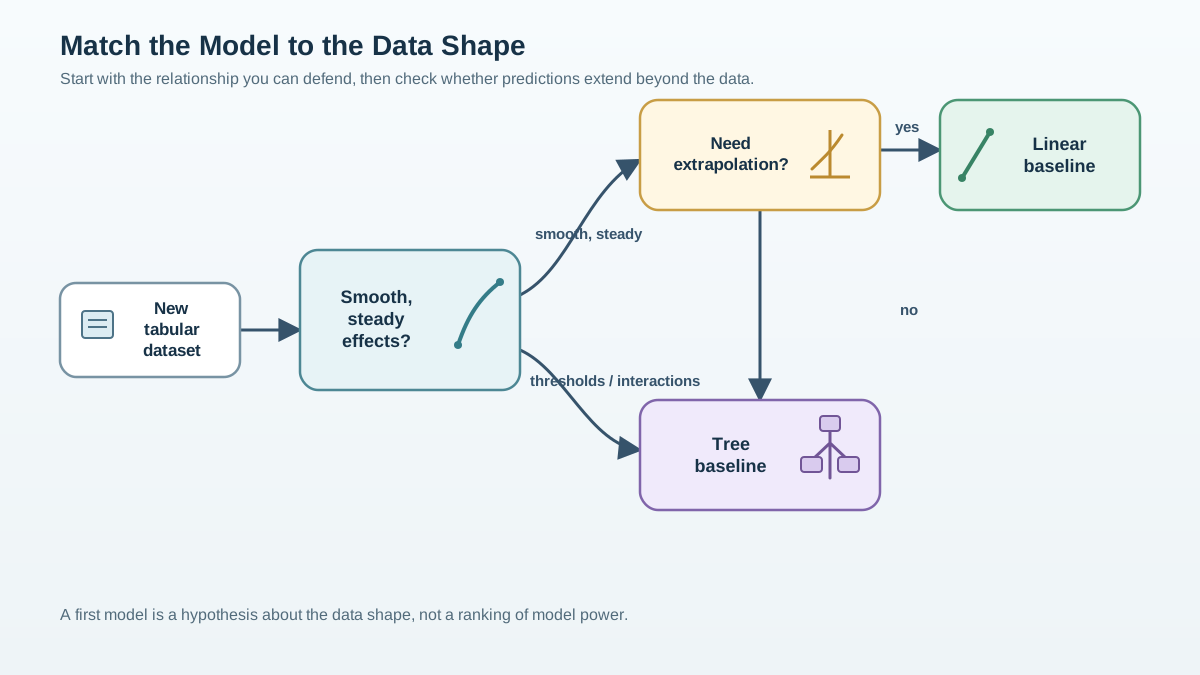
You now have the vocabulary. Here is the decision sequence I use when facing a new tabular dataset.
First, ask what shape the relationship plausibly has. If you expect smooth, steady effects—more experience means higher salary, larger apartment means higher rent—a linear model matches the shape. If you suspect thresholds, interactions, or irregular regions—credit risk that flips at certain income levels, disease risk that behaves differently across age bands—a tree matches the shape.
Second, ask whether you need to predict beyond the observed range. If you are forecasting next year's sales from this year's trend, you need extrapolation. That is a linear strength and a tree weakness. If you only need predictions inside the range of data you have seen, extrapolation is not a priority.
Third, ask how much you need to explain the prediction. Regulators, stakeholders, and your own debugging process often demand answers to "why this number?" Linear coefficients give you that directly. Trees give you readable rules, but a deep tree's rule path can become a maze.
My rule of thumb: start with a linear baseline when relationships look smooth and monotonic and you need interpretable coefficients or extrapolation. Reach for a tree when you suspect thresholds, interactions, or irregular shapes—and extrapolation is not on the table.
Then follow the baseline-first habit. Fit the simpler model first. Inspect its errors. The residual pattern will tell you whether a more flexible model earns its complexity. Do not skip this step because you suspect the data is nonlinear. The baseline gives you a reference point, and its failures tell you exactly which assumption is being violated.
Knowledge check
Check your understanding
Answer this question before you continue.
Diagnosing a Model's Blind Spots
No model family is wrong because it is weak. It is wrong because its assumptions do not match your data. The evidence of that mismatch shows up in predictable places.
For linear models, look at the residual plot—the difference between predicted and actual values. If you see a curve in the residuals, or systematic under-prediction at the extremes, the straight-line assumption is breaking. The model is telling you it cannot bend enough to follow the data.
For trees, watch for two signals. Flat predictions beyond the training range reveal the extrapolation limit. Unstable predictions from small changes in the training data reveal the variance problem—the tree is memorizing specific points rather than learning stable structure.
Treat these signals as evidence, not blame. The residual pattern is the model reporting which assumption it could not meet. Your job is to listen and respond.
The recovery moves are concrete. For a linear model failing on curvature, add polynomial features or interaction terms—or switch families. For a tree overfitting, control depth, raise the minimum leaf size, or move to an ensemble like a random forest.
When Neither Family Is the Whole Answer
Real workflows rarely end with a single plain tree or a bare linear regression. Ensembles—random forests and gradient boosting—fix the variance weakness of single trees and are often the practical default for tabular prediction. Hybrid ideas exist too: some models fit a linear regression inside each tree leaf, giving you local linear behavior inside a tree structure.
I mention these not to send you down a rabbit hole, but to close the loop. The point of this comparison was never to crown a winner. It was to give you the vocabulary to say which assumption your data is asking you to make. Once you can name that assumption, you can choose a model deliberately, diagnose its failures precisely, and know when a more complex family has actually earned its place.
Your Next Step
Take one dataset you care about. Fit a linear baseline. Plot the residuals. Look at the shape of the errors—are they random scatter, or do they curve and cluster?
That one plot will tell you more about your data than any model ranking. If the residuals look like noise, your linear model has done its job. If they show structure, you have found the exact shape a tree model might capture.
Fit the tree. Compare. Let the evidence decide.
Model choice is assumption-matching, not power-ranking. Start with the simplest model whose assumptions your data can honestly meet, and let its failures point you toward the next step. That habit will serve you longer than any default algorithm ever will.
Knowledge check
Final check
Finish the article by checking the ideas you just learned.
References
Research updated Sep 8, 2026


