Decision Trees Explained: How Splits Turn Features Into Rules

A decision tree is not a rulebook the model memorizes. It is a partitioning machine: a greedy process that keeps cutting your data into smaller, cleaner groups until each group is pure enough to make a prediction.

A Tree Is Not a Rulebook, It Is a Partitioning Machine

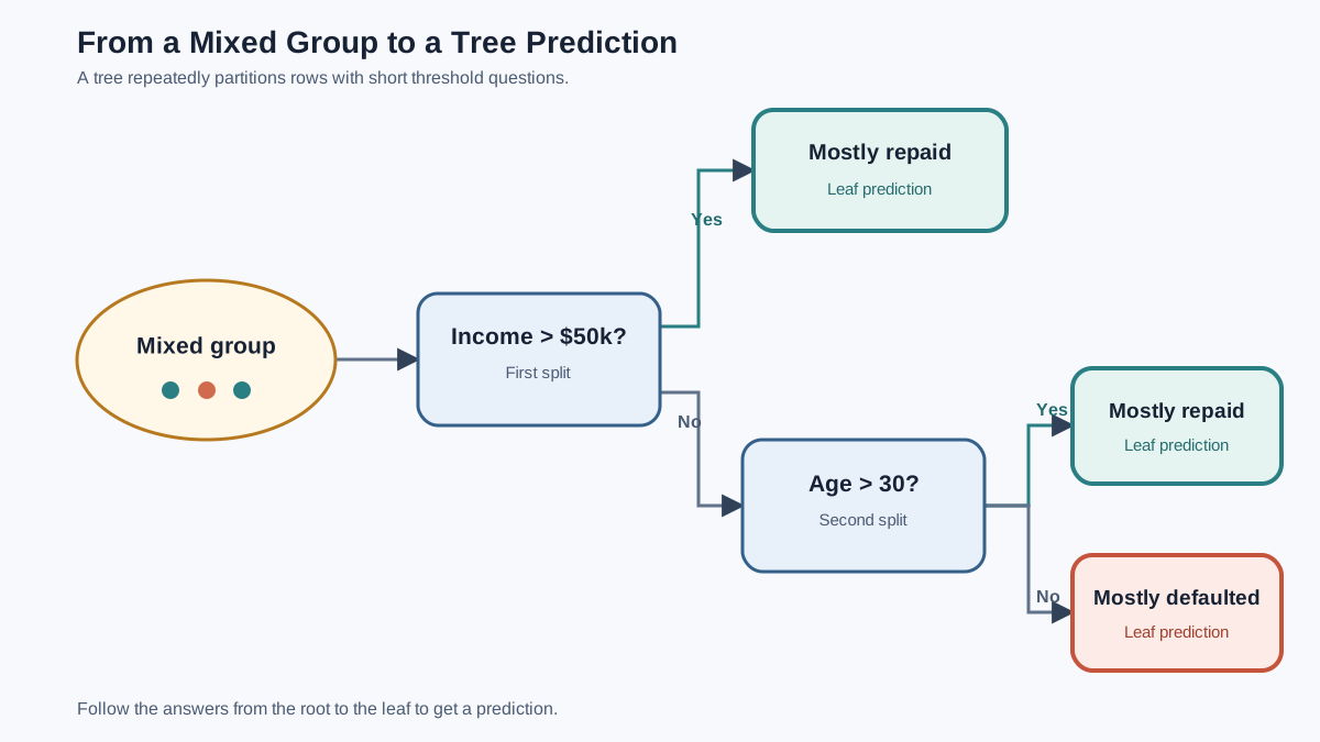
Here is a common misconception: a decision tree "learns rules" the way a human expert might write them down. It does not. The tree never steps back and thinks, "People with high income and low debt are good loan risks." Instead, it does something simpler and more mechanical: it repeatedly asks yes/no questions that divide your data into smaller groups.

Think about how you decide whether to bring an umbrella. You might first ask, "Is it raining right now?" If yes, you grab one. If no, you ask, "Are the clouds dark?" If yes, you bring it just in case. If no, you leave it. Each question splits the possibilities into two branches, and each answer narrows the decision.

A decision tree in machine learning works the same way, except the questions come from your data. Each question tests one feature against a threshold: "Is income above $50,000?" or "Is age over 30?" The answer sends a row of data down one branch or another.

The vocabulary is straightforward:

• Root node: the first question at the top of the tree, where all data starts.
• Internal node: any question in the middle of the tree.
• Leaf: an endpoint that makes the final prediction.
• Branch: the path a row travels based on its answers.
• Depth: how many questions a row must answer before reaching a leaf.

The tree keeps splitting until the groups are pure enough or a stopping rule fires. That is the whole mechanism. No hidden rulebook. Just cuts, repeated until the groups tell a clear story.

What Makes One Split Better Than Another

If the tree is just cutting data, how does it decide where to cut? It looks for the split that leaves both resulting groups cleaner than the parent group was.

Imagine you have a small dataset of loan applicants labeled "repaid" or "defaulted." Your root group is mixed: about half repaid, half defaulted. You want to ask the question that separates those two types as much as possible.

Consider two candidate splits. Split A asks about income above $50,000. The high-income group contains mostly repaid borrowers; the low-income group is still mixed. Split B asks about the applicant's favorite color. Both resulting groups remain just as mixed as the parent. Split A is clearly better because it made the groups more uniform.

That uniformity has a name: impurity. A group is pure when most members share the same target value. A group is impure when it is a jumble of different outcomes.

The scoring function scikit-learn uses by default is called Gini impurity. You do not need the formula to understand the idea. Think of Gini impurity as answering this question: if you randomly picked a person from a group and then randomly guessed their label based on the group's mix, how often would you be wrong? A perfectly pure group scores zero because you would never be wrong. A fifty-fifty group scores high because you would be wrong half the time.

The tree evaluates many candidate splits and picks the one that most reduces impurity. But here is the crucial detail: it is greedy. At each node, it picks the single best split for that moment, without planning ahead. It does not ask, "If I make this slightly worse split now, will it enable a much better split two levels down?" It takes the best immediate cut and moves on. Greedy works surprisingly well, but it means the tree is optimizing locally, not globally.

Reading a Tree: From Root to Leaf

Once a tree is trained, making a prediction is just following a path. Start at the root, answer each question using the row's feature values, and follow the branch until you hit a leaf.

What does the leaf tell you? For classification, the leaf records the class mix of the training samples that landed there, and the prediction is the majority class. If 40 defaulted borrowers and 10 repaid borrowers ended up in one leaf, the tree predicts "defaulted" for any new row that follows that path. For regression, the leaf predicts the average value of its training samples.

Here is an important point that surprises beginners: a mixed leaf is not an error. It is the tree admitting it could not separate those cases further with the features it had. The mix ratio tells you how the training data landed, but it is not a guarantee about new rows. A pure leaf—where every training sample shares one class—describes those training samples perfectly. It does not promise the same for a row the tree has never seen. That is why you judge a tree by how it performs on new data, not by how clean its leaves look.

When you inspect a trained tree, you can literally read the decision path: "Income above $50,000? Yes. Age above 30? Yes. Previous purchases? Yes. Prediction: will buy." That readability is the tree's superpower, and it is why decision trees are still used in fields where you must explain every prediction to a stakeholder.

Depth, Leaf Size, and the Overfitting Tradeoff

Here is where the tree's simplicity becomes a trap. A tree can always split further. Give it enough depth, and it will carve your training data into tiny pockets, each containing one or two samples. It will find a question that isolates every single training row perfectly.

That is overfitting: the tree has memorized the training data instead of learning patterns that generalize. To generalize means to perform well on new rows the model has not seen before. A depth-100 tree on a small dataset will achieve near-perfect training accuracy and then fail on new data, because it has learned the noise and accidents of the training set, not the underlying signal.

Two hyperparameters control this tradeoff:

• max_depth: a hard stop on how many questions a path can ask. Depth 3 means every prediction path involves at most three splits. The tree cannot chase noise beyond that limit.
• min_samples_leaf: a rule that forbids leaves with too few samples. If a split would create a leaf with fewer than the minimum, the tree refuses that split and stops early.

My practical advice: start shallow and inspect. Train a tree with max_depth=3, visualize it, and read the questions it chose. Then grow it carefully and watch what changes. If training accuracy climbs while validation accuracy stalls or drops, the tree has started memorizing. Pull the depth back or raise the minimum leaf size.

Common mistake: Judging a tree by its training accuracy. A tree can always memorize its training rows if you let it grow deep enough. The number that matters is how it performs on data it has not seen.

Why Noisy Features and Small Data Fool Trees

Trees have a specific weakness that is worth understanding before you trust one. On a small dataset, a noisy or irrelevant feature can look informative by pure chance.

Suppose you have 50 training rows and 200 features, most of them meaningless. By random luck, some meaningless feature will correlate with your target in those 50 rows. The tree does not know the feature is noise. It sees a split that reduces impurity and grabs it. With enough meaningless features, the tree will always find accidental patterns—there is always some pattern to find when the data is sparse and the feature space is wide.

This is why trees are unstable. Stability here means something specific: how much the learned model changes when the training data changes. A stable model changes little; an unstable one changes a lot. Change a few training rows, and the tree may choose entirely different splits at the top. The structure you admired yesterday can collapse and rebuild differently today because the greedy algorithm is sensitive to which samples happen to be present.

If your dataset is small or feature-heavy, expect a single tree to overfit. Constrain it with depth and leaf limits, or plan to combine many trees into an ensemble—which is exactly what random forests and gradient boosting do. They trade the single tree's readable structure for stability and accuracy.

When a Single Tree Is the Right Tool

Given all these weaknesses, when should you actually use a single tree?

Use one when interpretability matters more than peak accuracy. If you need to explain a decision path to a loan applicant, a doctor, or a regulator, the tree's readable structure is invaluable. You can point to the exact questions that led to a prediction. But keep that tree shallow and constrained. A depth-50 tree is technically inspectable and practically unreadable—the interpretability advantage evaporates as the tree grows bushy.

Use one when you want a quick, human-readable baseline before trying more complex models. A shallow tree tells you which features matter and gives you a sanity check for later models.

Do not rely on a single tree when you need top accuracy or stability. That is the domain of ensembles. And do not assume a single tree is always the simplest option—on wide, noisy datasets, it can quietly become one of the most overfit models you train.

One genuine practical advantage: trees handle numeric features with minimal preprocessing. You do not need to scale them or engineer elaborate transformations. The tree just finds thresholds. Categorical features are a different story—how the tree handles them depends on the estimator and how you encode them, so check your library's behavior rather than assuming every categorical column works as-is.

Your Next Step: Train a Tree and Watch It Think

The fastest way to make this mental model stick is to train a small tree and inspect it. Pick a familiar dataset, fit a tree with max_depth=3, and print or plot the tree structure. Read every question. Follow several rows from root to leaf and check whether the leaf predictions make sense.

Then change one thing at a time. Increase max_depth step by step, and watch what happens to training performance versus validation performance. The goal is not to hit a specific depth number. It is to find the point where training performance keeps improving while validation performance stops improving or starts falling. That gap is the overfitting signal. Raise min_samples_leaf and watch the tree prune itself back. Compare the two performance curves at each setting, and the tree will stop being a black box.

That instability you just observed is not a flaw to fix by tuning harder. It is the signal that a single tree has reached its limit—and the reason the next step is ensembles, where many constrained trees vote together to trade a little readability for a lot of stability.

References

Research updated Sep 8, 2026