
Linear Discriminant Analysis: Derive the Gaussian Classifier
You fit LinearDiscriminantAnalysis, plot the boundary, and get a straight line. Then someone asks why it is straight, and the honest answer is "because the…

Key topics
You fit LinearDiscriminantAnalysis, plot the boundary, and get a straight line. Then someone asks why it is straight, and the honest answer is "because the library says so." That is not understanding. That is a magic trick you happen to be holding.
Here is the stronger model: LDA is a generative Gaussian classifier. It assumes each class is a cloud of points drawn from a Gaussian distribution, and that all clouds share one covariance matrix. The straight boundary is not a design choice. It is a consequence of that single shared-covariance assumption. Everything below is the algebra that turns the assumption into the line.
Why a Gaussian Model Produces a Straight Line
LDA takes a generative stance. Instead of modeling the decision boundary directly, it models the class-conditional distribution and uses Bayes' rule to turn that into a decision. If you have already worked through the generative-versus-discriminative distinction, this is the same fork in the road: model the data, then derive the decision.
The setup is simple. For each class , assume the data comes from a multivariate Gaussian with mean and covariance . Bayes' rule gives the posterior:
You pick the class with the largest posterior. That is the whole classifier.
Now the central claim: when every class shares one covariance matrix , the quadratic terms in the posterior cancel, and the comparison collapses to a linear function of . The boundary between any two classes becomes a hyperplane.
QDA is the sibling that keeps per-class covariances . It keeps the quadratic terms, and its boundary curves. LDA is the special case where those terms vanish.
Notation and Assumptions Before the Algebra
Define the symbols once so the derivation reads cleanly.
| Symbol | Meaning |
|---|---|
| feature vector for one sample | |
| class label, | |
| mean of class | |
| shared covariance matrix, | |
| class prior | |
| posterior probability |
Four assumptions are doing real work here:
- Class-conditional Gaussianity. Each class's features follow a Gaussian. This gives the exponential form that later becomes a quadratic.
- Shared covariance (homoscedasticity). for all . This is the assumption that kills the quadratic term.
- Full-rank . The inverse must exist. If features are collinear or you have more features than samples, it does not.
- Priors from training frequencies. is estimated as the fraction of training samples in class .
These are claims about the data-generating process, not implementation details. When you call the estimator, it estimates , , and the priors from your training set, then plugs them into the formula we are about to derive.
From Bayes' Rule to the Log Posterior
Start with the posterior and drop the evidence term. Since does not depend on , it is identical for every class and cannot change the argmax:
Now substitute the multivariate Gaussian density for :
The exponent contains a Mahalanobis distance: how far is from , measured in units of the covariance. That distance is the heart of the classifier.
Take the log. The exponential disappears, products become sums, and the normalizing constant becomes an additive term:
Here collects the terms that do not depend on : the and the . Because is shared, is the same for every class, so it folds into and disappears from the comparison. Keep visible for one more step. It is about to do its job.
Knowledge check
Check your understanding
Answer this question before you continue.
Where the Quadratic Term Cancels
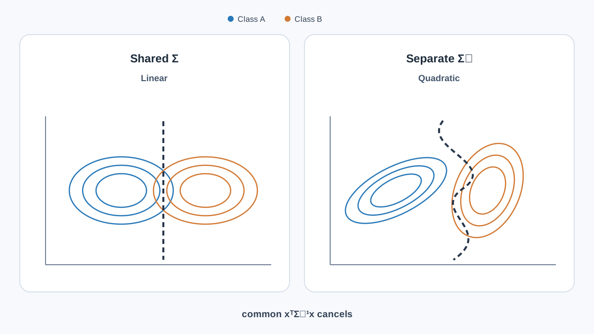
This is the single algebraic move that makes LDA linear. Expand the Mahalanobis term:
Look at each piece:
- contains no . It is the same for every class.
- is linear in , and it depends on through .
- is a constant per class.
Substitute this back into the log posterior. The term is identical for every class, so it cannot change which class wins the argmax. Drop it, along with the other class-independent constants, and collect what remains:
What survives is linear in . Define the weight vector and offset:
The score is now a clean linear function:
Assign to the class with the largest . Because each score is linear, the set of points where two scores are equal is a hyperplane. That is the LDA decision boundary, and it is straight for exactly one reason: the shared covariance made the quadratic term cancel.
Knowledge check
Check your understanding
Answer this question before you continue.
Reading the Score: Means, Covariance, and Priors
The formula is short enough to hold in your head. Each piece has a job.
The mean term. points the score toward class 's center, but stretched by the inverse covariance. In the sphered space where , this reduces to plain Euclidean distance to the mean. LDA is, at bottom, a nearest-mean classifier under a learned metric.
The covariance. reweights feature directions. Directions with small variance get large weight, because a small deviation there is informative. Directions with large variance get down-weighted. This is the model's built-in scale handling: a feature measured in the thousands is not automatically more influential than one measured in fractions, because the inverse covariance rescales each direction by its spread. What still bites in practice is estimation. When features are nearly collinear, or when the sample size is small relative to the number of features, the estimated becomes unstable and the weights swing wildly. That is a data problem, not a units problem, and shrinkage or regularization of the covariance is the fix.
The priors. shifts the offset. A more likely class gets a higher baseline, so the boundary slides toward the less likely class. With equal priors, the boundary sits at the midpoint in Mahalanobis space. Change a prior, and the line translates without rotating.
There is a clean geometric reading of all this: sphere the data so the covariance becomes the identity, then classify by nearest mean in Euclidean distance, adjusted by the log prior. The sphering step is what turns a tilted, stretched Gaussian cloud into a symmetric ball.
Knowledge check
Check your understanding
Answer this question before you continue.
A Worked Two-Class Example
Take two classes in two dimensions. Suppose:
With , the inverse is the identity, so . The scores are:
Set the priors equal. The term is zero, and the boundary is where :
That is the perpendicular bisector between the two means. Now make class 2 rarer: , . The log ratio is , so the boundary becomes:
The line slid toward class 2. Same orientation, new intercept. That is the prior doing its work: it makes the classifier demand more evidence before committing to the rare class.
Now change the covariance to . The inverse is , so the first feature is down-weighted. The weight vector rotates, and the boundary tilts. The covariance controls orientation and scale; the priors control position.
You can verify the hand result against the library in a few lines:
import numpy as np
from sklearn.discriminant_analysis import LinearDiscriminantAnalysis

X = np.array([[0, 0], [2, 2], [0.5, -0.5], [2.5, 1.5]])
y = np.array([0, 1, 0, 1])

lda = LinearDiscriminantAnalysis(priors=[0.8, 0.2]).fit(X, y)
print(lda.coef_)        # weight vector, up to scale
print(lda.intercept_)   # offset, includes the log-prior shift
The coefficients will not match your hand calculation exactly, because the library estimates from four points rather than using the identity. But the structure is the same: a weight vector and an offset. Change the priors argument and watch the intercept move while the coefficients barely budge.
Knowledge check
Check your understanding
Answer this question before you continue.
When the Assumptions Break
The derivation is a diagnostic checklist. Each assumption, when violated, produces a specific failure.
Unequal covariances. The quadratic terms no longer cancel. Under the Gaussian model, the true boundary curves, and LDA fits a straight line through a curved problem. It underfits. QDA keeps the per-class covariances and recovers the curve, at the cost of estimating more parameters.
Non-Gaussian or multimodal classes. A single mean and covariance cannot represent a class with two clusters. The score will be confidently wrong in the tails, where the Gaussian assigns probability mass the data never had. The boundary may still be linear, but it is the wrong boundary for the data.
Near-singular . When features are nearly collinear or approaches the sample size, becomes unstable. Small changes in the data produce large swings in the weights. Shrinkage or regularization of the covariance is the standard fix.
Class imbalance. The priors dominate the offset. The boundary drifts toward the minority class. Sometimes that is exactly what you want; sometimes it is a silent failure that inflates accuracy while destroying recall on the class you care about.
Common mistake: Treating LDA as "just a linear classifier like logistic regression." LDA makes a strong generative assumption about the shape of each class. Logistic regression does not. That difference is why LDA can be more stable in small samples and more fragile when the Gaussian assumption is wrong.
When to Reach for LDA
Use LDA when the classes are roughly Gaussian, roughly equally spread, and your sample size is small relative to the number of features. The shared covariance is a strong, low-variance estimator, and strong assumptions buy stability when data is scarce. It also works as an interpretable baseline and as a dimensionality-reduction step before another classifier.
Do not reach for it as a default on complex nonlinear problems. If the linearity assumption is clearly wrong, the derivation above tells you exactly why, and that is your signal to move on.
Compared with logistic regression, the tradeoff is assumption versus flexibility. LDA assumes a generative model and can outperform logistic regression in small samples when that model holds. Logistic regression makes fewer distributional assumptions and is the safer default when you cannot justify the Gaussian shape.
The next time you fit LDA and get a straight line, you will know it is straight because one shared covariance canceled the quadratic term, and you will know which knob to turn to move it. Perturb the priors in the worked example and watch the intercept slide. Perturb the covariance and watch the boundary rotate. When the shared-covariance assumption finally breaks, the natural next steps are QDA and regularized discriminant analysis, both of which relax the assumption this derivation depends on.
Knowledge check
Final check
Finish the article by checking the ideas you just learned.
References
Build stronger machine learning foundations
Use structured resources to connect theory, scikit-learn workflows, and evaluation practice.


