
How Cumulative-Link Models Represent Ordered Outcomes
A satisfaction rating of 4 when the truth was 5 is not the same kind of mistake as predicting 1. Most models cannot tell the difference. This one can — but…

Key topics
A satisfaction rating of 4 when the truth was 5 is not the same kind of mistake as predicting 1. Most models cannot tell the difference. This one can — but only if you understand what the structure actually guarantees and what it leaves to you.
The Problem: Discrete Categories With a Direction
Suppose you collect satisfaction ratings on a 1–5 scale and train a multiclass classifier. The model learns five separate decision regions. When it predicts 4 and the truth is 5, it pays the same penalty as when it predicts 1 and the truth is 5. The order you carefully encoded into the labels disappears the moment training begins.
Now flip to the other extreme. Treat the same target as a plain regression problem. The model minimizes squared error and happily predicts 3.7. That number implies a precision the rating scale never had. Nobody circled 3.7 on the survey. Worse, the model now assumes the distance from 1 to 2 equals the distance from 4 to 5, which may or may not be true.
You already know when order matters and why treating ordered categories as arbitrary labels throws away information. The question here is different: what structure lets a model respect order without pretending the categories are measurements? The cumulative-link model is one answer, and it is worth understanding from the inside.
Notation and the Latent-Score Idea
Before the equations, define the pieces.
Let be the observed target, taking one of ordered values: . For a satisfaction survey, . Let be the feature vector for one example, and the coefficient vector the model will learn.
Now introduce the key object: a latent variable . It is an unobserved continuous score. You never see it. You only see which bin it fell into.
The causal chain is short:
- Features produce a score: .
- The score falls into one of bins.
- The bin becomes the observed label .
Picture a horizontal axis. Cutpoints slice it into five labeled regions. A feature vector pushes the score left or right along that axis. Wherever it lands determines the predicted category.
The latent score is a modeling convenience, not a claim that satisfaction is a physical quantity you could measure with a ruler. It gives the thresholds something continuous to cut. That is its entire job.
Knowledge check
Check your understanding
Answer this question before you continue.
From Score to Probability: The Cumulative Structure
Here is where the model earns its name. Instead of predicting the category directly, it models the probability of landing at or below each level.
Start with the latent model and the binning rule. The observed category is when the score falls between threshold and threshold . So the event "" happens exactly when the score is below :
Substitute the latent model:
Rearrange to isolate the noise term:
If follows a logistic distribution, the cumulative distribution function is the sigmoid. That gives the standard form:
This is the cumulative-logit or proportional-odds model. Swap the logistic distribution for a Gaussian and you get the probit variant. The link function is the only thing that changes.
To recover the probability of a single category, difference adjacent cumulative probabilities:
Because cumulative probabilities are non-decreasing in , these differences are guaranteed non-negative. That is not an accident; it is a structural property of the formulation.
A Worked Example
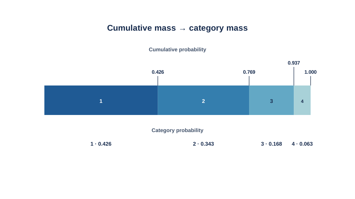
Take two features, one coefficient vector, and three thresholds. Let , , and thresholds , , for a four-level target.
First compute the linear predictor:
Now compute each cumulative probability:
Difference them to get category probabilities:
The four probabilities sum to 1. The predicted category is 1, but notice how the mass leans toward the lower end. A different shifts the whole distribution.
Knowledge check
Check your understanding
Answer this question before you continue.
What the Thresholds and Coefficients Actually Mean
The thresholds are cutpoints on the latent scale, not boundaries in feature space. They set the baseline split between adjacent levels. If you fit the model and find and , that tells you where the score axis gets sliced, not which feature values produce which category.
A coefficient shifts the entire latent score. A positive coefficient pushes the score rightward, moving probability mass toward higher categories. A negative coefficient does the opposite. In the worked example, the second feature has a negative coefficient, so increasing it lowers the score and shifts mass downward.
The single-coefficient-per-feature structure is the proportional-odds assumption. The effect of a feature is constant across all thresholds. There is no separate coefficient for "the transition from 2 to 3" versus "the transition from 4 to 5." One coefficient governs all of them.
This is the sharpest contrast with nominal multiclass classification. There, you get a separate score per class, each with its own coefficient vector. Here, you get one score plus ordered cutpoints. Fewer parameters, more structure, and a built-in respect for order.
Knowledge check
Check your understanding
Answer this question before you continue.
The Assumptions and What Breaks When They Fail
Every model is a set of bets. Here are the ones this model places.
Proportional odds. The feature effect is the same at every threshold. When it is not — when a feature strongly separates low categories but barely matters for high ones — the model underfits some transitions and overfits others. The single coefficient becomes a compromise that fits none of them well.
Independence of observations. Standard cumulative-link models assume each observation is independent. Grouped or repeated-measures data violates this and requires an extension with random effects.
Correct specification of the linear predictor on the latent scale. If the true relationship between features and the latent score is nonlinear, a linear predictor will miss it.
The latent score itself is a construct. The model does not prove that satisfaction is continuous or that the gaps between levels are equal. It assumes a continuous score exists and that the thresholds carve it into the categories you observe. That assumption may be wrong, but it often buys more than it costs.
Two failure modes deserve explicit warning. If the target is genuinely nominal — think color categories or unordered species — imposing order forces a structure the data does not support. The model will produce predictions, but the thresholds will be meaningless. If the target is truly continuous and you have the original measurements, binning into categories discards information that a regression model would have used. Do not throw away precision you already have.
Extensions like partial proportional odds relax the constant-effect assumption by allowing some features to have threshold-specific coefficients. Scale effects model the variance of the latent distribution. These exist, and they are useful, but they are not where you start.
Knowledge check
Check your understanding
Answer this question before you continue.
Why This Is Not Nominal Multiclass Classification
The structural difference is worth stating plainly, because it changes what the model can learn and how you should evaluate it.
| Nominal multiclass | Cumulative-link | |
|---|---|---|
| Objective | One score per class, normalized | One score plus ordered thresholds |
| Parameters | coefficient vectors | One coefficient vector plus thresholds |
| Output | Class probabilities | Cumulative probabilities, differenced to class probabilities |
| Order handling | None; classes are interchangeable | Built into the threshold structure |
| Typical failure | Wastes order information | Wrong when order is not real or effects vary by threshold |
The cumulative structure encodes order into the model itself. A wrong-but-close prediction is penalized less than a wrong-and-far one, because the latent score only needs to cross one threshold to reach the adjacent category. In nominal multiclass, crossing from class 1 to class 5 is the same distance as crossing from class 1 to class 2.
That last paragraph needs a correction, because it is the most common place to get this wrong. The threshold structure constrains how probabilities relate across categories. It does not, by itself, define the penalty your training objective or evaluation metric applies. If you train a nominal multiclass model with cross-entropy and evaluate it with accuracy, both mistakes cost the same. If you train a cumulative-link model and evaluate it with accuracy, both mistakes still cost the same. The order lives in the probability model, not in the loss.
To get distance-sensitive penalties, you have to choose them explicitly. Mean absolute error on the numeric labels treats a 1-off prediction as half the cost of a 2-off prediction. A quadratic weighted kappa or a distance-weighted confusion matrix does something similar. The cumulative-link structure makes those measures meaningful because the model's probabilities already respect order, but the structure does not enforce them for you.
This has an evaluation consequence. Accuracy alone hides whether the model respects order. A model that predicts 4 when the truth is 5 and a model that predicts 1 when the truth is 5 can have identical accuracy. Ordered error measures — mean absolute error on the numeric labels, or a confusion matrix that reveals the distance structure — show what accuracy conceals.
When to Reach for a Cumulative-Link Model
Use it when three conditions hold: the target is discrete, the categories have a meaningful order, and the levels are plausibly a coarse view of an underlying continuum. Satisfaction ratings, severity grades, Likert scales, and ordered risk tiers all fit.
Use it when you want one interpretable effect per feature. If you need to explain to a stakeholder how a one-unit increase in a feature shifts the odds of landing in a higher category, the single-coefficient structure gives you that answer directly.
Do not use it when the categories are unordered. Do not use it when the target is genuinely continuous and you can model it directly. And before trusting the single-coefficient structure, check whether the proportional-odds assumption is plausible on your data. A simple diagnostic: fit separate binary logistic models for each cumulative split and compare the coefficients. If they diverge substantially, the assumption is strained.
One practical note: scikit-learn does not ship a first-class cumulative-link estimator. This is a case where the theory tells you which tool to reach for. Libraries like statsmodels and the ordinal package in R implement these models directly. Knowing the formulation means you can evaluate whether the tool you find is implementing what you expect.
The mechanism is one sentence: a latent score plus ordered thresholds. Features push the score; thresholds slice it; the slice becomes the label. If your target is discrete and ordered, model the cumulative probability of landing at or below each level rather than fitting independent class scores. Then check whether the proportional-odds assumption holds before you trust the single-coefficient structure. That check is the difference between using the model and being used by it.
Your next step: take an ordered target you already have — a rating, a grade, a severity tier — and fit both a nominal multiclass baseline and a cumulative-link model. Compare them with accuracy, then with mean absolute error on the numeric labels. The gap between those two views will tell you whether the order in your data is real signal or just a label you typed in.
Knowledge check
Final check
Finish the article by checking the ideas you just learned.
References
Build stronger machine learning foundations
Use structured resources to connect theory, scikit-learn workflows, and evaluation practice.


