
Naive Bayes: Derive the Classification Score From Bayes' Rule
The intuition article told you Naive Bayes "combines prior and evidence." Then you tried to write $P(x_1, x_2, \dots, x_n \mid y)$ for real data, and the…

Key topics
The intuition article told you Naive Bayes "combines prior and evidence." Then you tried to write for real data, and the table exploded. This article is the escape hatch: start from Bayes' rule, watch the joint distribution become unmanageable, then let one assumption collapse it into a product of small one-dimensional pieces — and prove the result is a linear score in disguise.
Set Up the Notation Before the Algebra
Before any derivation, pin down the symbols. A derivation you can't read is just a formula wall.
- is the class variable. It takes one of values, written (or just when the context is clear).
- is the feature vector for one instance. Each is a single feature — a word count, a pixel, a measurement.
- Our goal: for a new instance , compute for every candidate class, then pick the class with the largest value.
Two quantities must be estimated from training data:
- The prior — how common each class is before you see any features.
- The class-conditional — how likely a feature vector is, given the class.
The prior is easy. The class-conditional is where the trouble starts. If you have binary features, the full joint needs a separate parameter for every one of the feature combinations. Twenty features means over a million parameters per class. Real datasets don't have that many rows, so most combinations never appear, and the estimate is mostly zeros.
If you've read the intuition piece on how Naive Bayes combines prior and evidence, you already know the "naive" label refers to an independence assumption. Here we do the actual algebra of that assumption and see exactly where it enters.
Start From Bayes' Rule and Watch the Joint Explode
Bayes' rule gives the posterior directly:
Each term has a job. is the prior. is the likelihood — the class-conditional. is the evidence: the probability of seeing this feature vector at all, regardless of class.
The evidence term expands as a sum over classes:
Notice what that means. does not depend on . It is the same number for every candidate class. That is the first hint it will not affect the decision — and it's the reason the denominator eventually drops out entirely.
Now the bottleneck. For binary features, the naive joint requires on the order of parameters to characterize. Under the independence assumption, you need only . The gap is not a constant factor; it is exponential versus linear. At , that's roughly two million parameters versus forty.
With finite data, the exponential version fails in a specific way: most feature combinations never appear in the training set, so their estimated probability is zero. A single zero in the joint wipes out the entire product. The classifier becomes useless — not because the math is wrong, but because the estimate has no data to stand on.
The assumption that rescues us is stated formally as:
In words: once you know the class, knowing every other feature tells you nothing extra about feature . That is the conditional independence assumption. It is almost always false in real data. We'll come back to why the classifier still works anyway.
Knowledge check
Check your understanding
Answer this question before you continue.
Factor the Likelihood With Conditional Independence
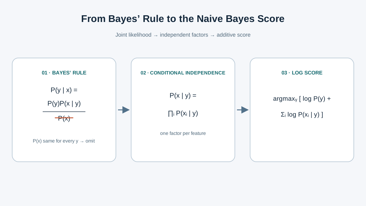
Here is where the assumption does its work. Start with two features and apply the chain rule — a general property of probability that holds regardless of any assumption:
Now substitute the independence assumption. The term simplifies to :
Generalize to features:
Substitute this back into Bayes' rule to get the fundamental Naive Bayes equation:
For classification, we only need the most probable class. Since is constant across classes, it drops out of the comparison:
This is the classification rule. Each is a one-dimensional distribution estimated independently from counts. That decoupling is why Naive Bayes tolerates small datasets: you are not estimating a joint over dimensions, you are estimating separate one-dimensional distributions.
The distribution you choose for defines the model variant. Gaussian for continuous features, multinomial for counts, Bernoulli for binary presence/absence, categorical for discrete values. The derivation above is the same for all of them; only the per-feature distribution changes.
Knowledge check
Check your understanding
Answer this question before you continue.
Why We Take Logs: From Products to Sums
The product form has a practical problem. Multiply enough small probabilities together and the result underflows to zero in floating point. With a few hundred features, every class scores zero and the argmax is meaningless.
The fix is to take the logarithm. Since is monotonically increasing, the argmax is unchanged:
The product became a sum. That single transformation gives you two things.
Numerical stability. Summing log-probabilities keeps the score in a usable range instead of collapsing to zero. Log-probabilities are measured in nats — units of information — and they add cleanly.
Structural clarity. The score is now a weighted sum of per-feature contributions plus a prior term. That is exactly the form of a linear classifier in log space. Each feature votes, the votes add up, and the class with the highest total wins. This is why Naive Bayes is fast, interpretable, and easy to inspect: you can read off which feature contributed most to a decision.
Common mistake: Dropping the prior term because "it's just a constant." The prior is constant across features, not across classes. It shifts the decision boundary and matters enormously when classes are imbalanced. A spam filter trained on 99% ham will predict ham for almost everything if you ignore the prior.
Warning: The log score is not a calibrated probability. It ranks classes correctly more often than it estimates their true likelihood. Do not treat the raw score as "the probability this email is spam."
Knowledge check
Check your understanding
Answer this question before you continue.
Work a Small Example by Hand
Let's classify whether a message is spam based on two binary features: contains "free" () and contains "meeting" (). Training data:
| Message | (free) | (meeting) | Class |
|---|---|---|---|
| 1 | 1 | 0 | spam |
| 2 | 1 | 1 | spam |
| 3 | 0 | 0 | ham |
| 4 | 0 | 1 | ham |
| 5 | 0 | 1 | ham |
Priors. Spam: . Ham: .
Class-conditionals with Laplace smoothing. Without smoothing, , and any message without "free" would score zero for spam regardless of other evidence. Add 1 to every count and 2 to every denominator (two possible values per feature):
Score a new message with ("free") and ("meeting").
Raw probability form:
Log form:
Both forms agree: spam wins. The log scores are negative because probabilities are below 1, but the comparison is what matters.
Read the numbers. The feature "free" contributed for spam versus for ham — a swing of over 1.3 nats. The prior gave ham a head start of about 0.4 nats, but "free" overwhelmed it. That is the mechanism: each feature adds evidence, and the class with the largest total wins.
Knowledge check
Check your understanding
Answer this question before you continue.
See What the Independence Assumption Actually Changes
The example above proves the arithmetic. It does not yet show what the assumption costs you. To see that, compare the factorized likelihood against the true joint on a feature pair that is deliberately dependent.
Suppose two features are "contains free" and "contains prize." In spam, these words travel together: a message with "free" usually also has "prize." In ham, they almost never co-occur. The training counts might give:
The factorized likelihood multiplies them:
But the actual class-conditional joint, read directly from the data, is:
The factorized model underestimates the joint by a wide margin. Why? Because it treats the two features as independent votes. In reality, "prize" adds almost no new evidence once you already know "free" is present — the two features are telling the same story. Naive Bayes counts that story twice, so its confidence is miscalibrated.
Now the crucial part. Suppose the ham joint for the same pair is . The factorized ham score is . Even though both factorized values are wrong, the ratio still favors spam by a wide margin. The ranking survives; the confidence does not.
That is the boundary the assumption draws. Conditional independence is a lie about the data, but it is often a lie that preserves the ordering of classes. When it does, Naive Bayes classifies well. When the dependence structure flips the ordering — for example, when two features are individually weak but jointly decisive for the wrong class — the classifier fails. The assumption is not "harmless." It is a bet that the ranking is robust to the distortion.
What the Assumption Does and Does Not Justify
The independence assumption is almost always false. Height and weight are not independent given sex. Word frequencies are not independent given topic. So why does Naive Bayes work?
Because classification only needs the ranking of classes to be correct, not the probabilities. Even when the posterior estimates are badly wrong, the argmax can still land on the right class. The errors from double-counting correlated features often cancel or reinforce the correct ranking.
Where the assumption bites:
- Correlated features get double-counted. If two features carry the same signal, the score overstates confidence. The predicted class may be right, but the probability is inflated.
- Posterior probabilities are not trustworthy. Use Naive Bayes for ranking and fast baselines, not for probability estimates you plan to act on directly.
- Smoothing is not optional. Without it, a single unseen feature value zeros out the entire product for that class. Laplace smoothing is the standard fix.
My rule: reach for Naive Bayes when you need a fast, interpretable baseline on text or high-dimensional sparse data, and you care about ranking more than calibration. Reach for a discriminative model like logistic regression when you need calibrated probabilities or when features are strongly correlated and you can afford the training cost.
Prove It to Yourself
The derivation is short enough to hold in your head, but holding it is not the same as owning it. Two exercises will close the gap.
First, re-derive the two-feature case from memory. Write Bayes' rule, apply the chain rule, substitute independence, take the log. If you can do it without looking, the mechanism is yours.
Second, implement the log-score rule in a few lines of NumPy on the toy data above, then compare your predictions against scikit-learn's CategoricalNB on the same table. When your hand-computed scores match the library's output, you have proven the theory to yourself — and you will never again treat the formula as something you merely recognize.
Knowledge check
Final check
Finish the article by checking the ideas you just learned.
References
Build stronger machine learning foundations
Use structured resources to connect theory, scikit-learn workflows, and evaluation practice.


