
Naive Bayes Explained: How Simple Probability Can Classify Well
Most classifiers earn their keep by capturing relationships between features. Naive Bayes does the opposite: it assumes those relationships don't exist.…

Key topics
Most classifiers earn their keep by capturing relationships between features. Naive Bayes does the opposite: it assumes those relationships don't exist. And then it wins anyway.
That's the strange truth about this algorithm. The "naive" assumption—that every feature is independent of every other feature given the class—is almost always false in real data. Spam emails that contain the word "free" are also more likely to contain the word "money." Documents about baseball tend to mention "run" more often than documents about cooking. The features are correlated, and naive Bayes simply ignores that correlation.
Yet this deliberately oversimplified model remains one of the most practical tools in the classical machine learning toolbox. It powers spam filters, classifies documents, and handles high-dimensional text data with ease. It trains in a blink, needs surprisingly little data, and often performs competitively against far more sophisticated models.
The key to understanding naive Bayes is to stop expecting it to model the true relationships in your data. Instead, think of it as a fast evidence counter: each feature contributes a piece of class-specific evidence, and the model multiplies those pieces together to reach a verdict. When many weak signals point the same direction, naive Bayes is hard to beat.
Bayes' Rule: Flipping the Question You Can Answer
Before we get to the evidence-accumulation mechanism, we need the engine underneath it: Bayes' rule.
Here's the problem naive Bayes solves. You have an email and you want to know: given the words in this email, what is the probability it's spam? In probability notation, that's P(spam | words)—the probability of the class given the features.
The trouble is that this quantity is genuinely hard to estimate directly. There are too many possible combinations of words to count them all reliably.
Bayes' rule gives us a way to flip the question into pieces we can estimate from data:
P(class | features) = P(features | class) × P(class) / P(features)
Each piece has a plain-language meaning:
- Prior — P(class): How common is this class overall? If 20% of all emails are spam, the prior for spam is 0.2.
- Likelihood — P(features | class): If an email is spam, how likely are these particular words? This is the evidence each feature contributes.
- Evidence — P(features): How common are these features across all emails, spam or not? This is a normalizing constant.
- Posterior — P(class | features): The answer we actually want. Given what we observed, how likely is each class?
The elegant trick is that Bayes' rule lets us invert a question we can't answer directly into questions we can answer by counting. We don't need to know how often "free" appears in spam and how often spam appears given "free." We just need to know how often "free" appears within spam, and how often spam appears overall.
Knowledge check
Check your understanding
Answer this question before you continue.
The Naive Assumption: Why "Naive" Is Actually a Feature
Now we hit the assumption that gives the algorithm its name.
To compute P(features | class) properly, we'd need to know how all the features interact within each class. With just 20 binary features, that means estimating over a million joint probabilities. With the thousands of words that appear in a typical text classification problem, the full model becomes computationally impossible.
The naive assumption collapses this explosion: given the class, every feature is independent of every other feature. Knowing that an email contains "free" tells you nothing extra about whether it also contains "money"—once you already know it's spam.
Mathematically, this turns one giant joint probability into a product of small per-feature probabilities:
P(features | class) = P(feature₁ | class) × P(feature₂ | class) × ... × P(featureₙ | class)
Instead of estimating one enormous table, we estimate one small probability per feature per class. With n binary features, the full model needs an exponentially growing table of joint probabilities, while naive Bayes needs only a linear set of per-feature estimates. That factorization is why naive Bayes survives high-dimensional text data: it never asks the data to fill in a table that would dwarf the number of training examples available.
Here's a useful way to picture it: imagine each feature as a witness testifying about the class. One witness says "the word 'free' appears—that points toward spam." Another says "the word 'meeting' appears—that points toward legitimate." Naive Bayes treats each witness's testimony as independent evidence, then combines all the testimony to reach a verdict. It never tries to model how the witnesses might influence each other.
But there's a crucial detail that separates this from a simple vote: the witnesses don't cast equal votes. Each feature's contribution is weighted by how much more likely it is under one class than the other. A word that appears in 70% of spam but only 10% of legitimate email is a strong witness. A word that appears equally often in both classes is a useless witness—it carries no information, no matter how frequently it appears.
That sounds like a weakness, and conceptually it is. But here's the practical payoff: because the model is so simple, it needs very little data to estimate its parameters, it trains extremely fast, and it doesn't suffer from the curse of dimensionality the way more complex models do. The naive assumption isn't a bug that naive Bayes tolerates—it's the design choice that makes the algorithm work at all.
Knowledge check
Check your understanding
Answer this question before you continue.
How Evidence Accumulates: From Likelihoods to a Verdict
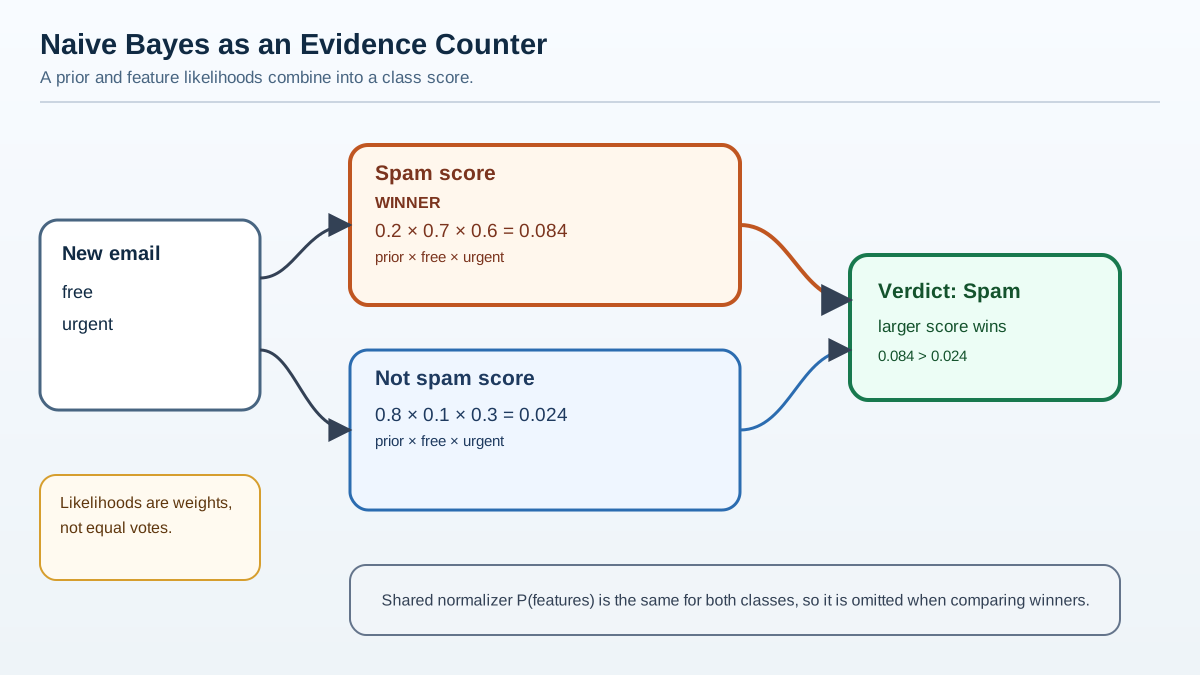
Let's walk through the actual decision process with a small example.
Suppose we're classifying emails as spam or not spam using just two words: "free" and "urgent." From our training data, we've estimated:
- Prior: 20% of emails are spam, 80% are not.
- Likelihoods for spam: 70% of spam contains "free," 60% contains "urgent."
- Likelihoods for not spam: 10% of legitimate email contains "free," 30% contains "urgent."
A new email arrives containing both words. Which class wins?
For spam: 0.2 × 0.7 × 0.6 = 0.084 For not spam: 0.8 × 0.1 × 0.3 = 0.024
Spam wins by a comfortable margin. The prior started against spam, but the feature evidence—both words appearing—overwhelmed it.
Now look at why each word mattered. "Free" is the stronger witness: it's seven times more likely in spam than in legitimate email. "Urgent" is weaker: only twice as likely in spam. If the email had contained only "free," spam would still win. If it had contained only "urgent," the prior would have kept not-spam ahead. The evidence isn't counted in equal votes—it's weighted by how sharply each feature discriminates between classes.
Notice what we didn't compute: the denominator P(features). That's because the evidence is the same for every class. It's a normalizing constant that ensures probabilities sum to 1, but it doesn't change which class has the highest score. When we only care about the winner, we can drop it and compare the numerators directly.
One practical detail matters at scale. When you multiply hundreds of small probabilities together, the product underflows to zero in floating-point arithmetic. That's why real implementations work in log space: instead of multiplying probabilities, they add logarithms. The class with the highest log-score is the same class that would win the multiplication—but the arithmetic stays numerically stable.
Common mistake: Don't confuse the naive assumption with a claim that your features are actually independent. The model assumes independence to make the math tractable; it doesn't verify it. If two features are really the same signal in disguise—say, "free" and "free!!!"—the model may count that evidence twice, inflating its confidence. The classification can still be useful, but the reported probabilities will be overconfident.
Knowledge check
Check your understanding
Answer this question before you continue.
Three Flavors for Three Data Types
Naive Bayes isn't a single algorithm but a family. The core mechanism stays the same; what changes is how each flavor models P(feature | class). Scikit-learn exposes three main variants:
| Variant | Feature type | What it estimates |
|---|---|---|
| GaussianNB | Continuous values | A bell-shaped (normal) distribution per feature per class, defined by its mean and variance |
| MultinomialNB | Integer counts | How often each word or event appears, most famously word counts in text |
| BernoulliNB | Binary values | Whether a word is present or absent, not how many times it appears |
The rule of thumb is straightforward. Continuous measurements like height, temperature, or sensor readings? Use GaussianNB. Text data where you're counting word occurrences? MultinomialNB. Text data where you only care whether a word appears at all? BernoulliNB.
All three follow the same scikit-learn interface: call fit(X, y), then predict(X). The choice between them comes down to matching the flavor to your feature type.
Knowledge check
Check your understanding
Answer this question before you continue.
When Naive Bayes Earns Its Place (and When It Doesn't)
The honest question is when this deliberately naive model deserves a spot in your workflow. Here's the practical test I use: don't try to prove that your features are conditionally independent—you usually can't, and you don't need to. Instead, run the comparison and let validation tell you.
Use naive Bayes when:
- Your data is high-dimensional and sparse. Text classification is the classic case. With millions of possible words as features, naive Bayes trains quickly because its parameters are just per-feature, per-class estimates—no interaction terms to fit.
- You have little training data. The simple model needs few parameters to estimate, so it doesn't demand large datasets.
- You need a fast, interpretable baseline. Naive Bayes is often the first real model to try after a majority-class baseline. If it performs well, you may not need anything more complex.
Skip naive Bayes when:
- You need calibrated probabilities. Scikit-learn's documentation puts it plainly: naive Bayes is a decent classifier but a bad probability estimator. The ranking of classes is usually reliable, but the raw probabilities from
predict_probashould be treated with skepticism. - Your features are near-duplicates of each other. If you've created many features from the same underlying signal, naive Bayes may count that signal repeatedly and become overconfident. Feature selection or a different model may serve you better.
The comparison workflow: Fit a majority-class baseline, then a naive Bayes model, then a logistic regression, using the same validation split or cross-validation for all three. Compare class-level metrics, not just overall accuracy. If naive Bayes matches logistic regression, you've saved yourself complexity. If it falls short, the gap tells you something real about your data—but not necessarily that interactions are the culprit. The gap could come from duplicated features, a poor distribution match, or a representation that simply doesn't fit the naive assumption.
My rule is simple: naive Bayes is the first real model I try on high-dimensional problems, especially text. It sets a baseline that more complex models have to beat. When it performs well, I've saved myself a lot of complexity. When it performs poorly, the failure mode is informative—it tells me the representation deserves scrutiny, and it points me toward models that can capture feature relationships.
The Mental Model That Sticks
Here's the durable image to carry forward: naive Bayes is a fast evidence counter. Each feature contributes a class-specific likelihood, those likelihoods get multiplied together, and the class with the strongest combined evidence wins. It doesn't try to understand how features influence each other—it just weighs each piece of evidence on its own and picks a winner.
That simplicity is both its strength and its boundary. It wins when many weak signals point the same way and the cost of modeling every interaction isn't justified. It struggles when the real signal lives in feature combinations, or when related features inflate its confidence.
The best way to internalize this is to run the experiment yourself. Pick a small text dataset, fit a MultinomialNB in scikit-learn, and compare it against a majority-class baseline and a logistic regression. Observe where the gap appears and where it doesn't. That comparison will teach you more about when naive Bayes earns its place than any theoretical discussion.
And when you're ready to push further, the natural next question is how naive Bayes differs from logistic regression at a deeper level. Naive Bayes models how features are produced within each class, then uses Bayes' rule to flip that around into a classification decision. Logistic regression skips the feature-generation story and draws a boundary between classes directly. That contrast—modeling the classes versus modeling the boundary—explains why the two models behave differently, and why each earns its place in your toolbox.
Knowledge check
Final check
Finish the article by checking the ideas you just learned.
References
Research updated Sep 8, 2026


