
Derive Softmax Probabilities and the Multiclass Cross-Entropy Objective
A multiclass model hands you K raw scores. The obvious move — divide each by their sum — collapses the first time a score goes negative. Here is the fix,…

Key topics
A multiclass model hands you K raw scores. The obvious move — divide each by their sum — collapses the first time a score goes negative. Here is the fix, and where the loss function actually comes from.
From Binary Logits to K Class Scores
You already know the binary case. A linear model produces one score, the sigmoid squashes it into a probability, and the complement gives you the other class. One score, one probability, one decision.
Multiclass problems break that symmetry. With K classes, there is no "the other class" to fall back on. So we give every class its own parameters. For class , with weight vector and bias :
Stack the results into a vector . These are logits — raw, unnormalized scores. They can be negative, they can be huge, and they do not sum to anything meaningful. A logit of does not mean "42% likely." It means nothing on its own.
Our goal is a map from to a probability vector where every and . Two properties matter: the map should be monotonic (a larger score must produce a larger probability) and differentiable (so gradient-based optimization can find the weights).
Knowledge check
Check your understanding
Answer this question before you continue.
Why Naive Normalization Fails
The tempting candidate is . Try it on . The denominator is , and you get . That is not a probability distribution. It has a negative entry, and it sums to only by accident.
Two requirements are violated at once: non-negativity, and a denominator that is guaranteed positive. If all scores are negative, the denominator flips sign and every "probability" inverts.
We need a transformation that is always positive and strictly increasing. The exponential is the smallest such change: for every real , and it preserves order. Apply it, then normalize.
Knowledge check
Check your understanding
Answer this question before you continue.
Deriving the Softmax Function
Two steps, each fixing one broken requirement.
Step 1 — guarantee positivity. Replace each score with . Every term is now strictly positive.
Step 2 — guarantee the sum is 1. Divide each term by the total:
That is the softmax function. The name comes from the fact that it is a smooth approximation of argmax: push one score far above the rest and its probability approaches 1 while the others approach 0.
Check the two properties. Each is a positive number divided by a sum that is larger than it, so . And the numerator of the whole vector sums to exactly the denominator, so . Both requirements hold.
Note: With , softmax reduces to the sigmoid. Let and factor out : you get , which is the sigmoid applied to the score difference. That is the check that softmax is a genuine generalization, not a separate invention.
One practical detail. Exponentials overflow fast — is not a number your machine will store. The standard fix is to subtract the maximum score before exponentiating:
This changes nothing mathematically, because the same factor cancels from numerator and denominator. It just keeps the largest exponent at .
That cancellation is not a coincidence. It reveals that softmax is shift-invariant: add any constant to every score and the output is identical. Only score differences carry information. This redundancy is a real modeling fact, not a curiosity — it is why one class's weights can be treated as a reference, and why the parameters are not uniquely identified without regularization.
Knowledge check
Check your understanding
Answer this question before you continue.
From Scores to a Likelihood
So far softmax is just a mapping. To get a loss function with a principled origin, we need a probabilistic model.
Assume that given input , the label is drawn from a categorical distribution with probabilities . Encode the true label as a one-hot vector , where for the correct class and elsewhere.
The probability of observing the correct label is then:
Every factor where contributes . The single factor where selects the predicted probability of the true class. The one-hot encoding turns a product over all classes into a lookup.
For a dataset of examples, the likelihood is the product of per-example likelihoods:
This factorization assumes the examples are conditionally independent given their features. That assumption is about the dataset, not about the categorical model itself. When examples are genuinely dependent — successive tokens in a sentence, consecutive frames in a video — you cannot factor the joint likelihood this way, and you need a model that represents the dependence. The per-example categorical loss still shows up inside those models; it just gets combined with a sequence structure rather than multiplied naively across independent rows.
We want to maximize this quantity — the parameters that make the observed labels most probable are the ones we keep. But products of many small probabilities underflow to zero, and products are awkward to differentiate. So we take the log next.
Knowledge check
Check your understanding
Answer this question before you continue.
Deriving the Cross-Entropy Objective
The log turns the product into a sum:
The inner sum over classes collapses again, because only one is nonzero. For each example, you are left with a single term: the log-probability of the true class.
Maximizing a sum is the same as minimizing its negative. Flip the sign:
This is the negative log-likelihood, and it is also the cross-entropy between the one-hot target distribution and the predicted distribution. Averaging over examples gives the per-example loss that scikit-learn minimizes for multinomial logistic regression.
Read the loss value directly. It is the negative log-probability assigned to the correct class. Assign probability to the right answer and the loss is . Assign probability and the loss is about . As that probability approaches zero, the loss grows without bound. The objective punishes confident wrong answers hardest, which is exactly what you want.
A Worked Example by Hand
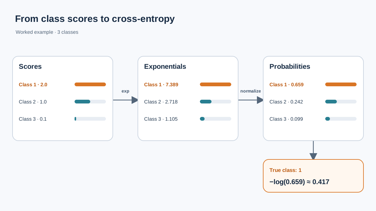
Take three classes and the score vector .
| Class | Score | Probability | |
|---|---|---|---|
| 1 | 2.0 | 7.389 | 0.659 |
| 2 | 1.0 | 2.718 | 0.242 |
| 3 | 0.1 | 1.105 | 0.099 |
The denominator is . Dividing each exponential by it gives , which sums to .
Suppose the true class is class 1. The loss is .
Now make the model confidently wrong. Use , where class 2 dominates but class 1 is the truth.
| Class | Score | Probability | |
|---|---|---|---|
| 1 | -1.0 | 0.368 | 0.026 |
| 2 | 3.0 | 20.086 | 0.943 |
| 3 | 0.5 | 1.649 | 0.077 |
The loss is — nearly nine times larger. The model assigned almost no probability to the correct answer, and the objective says so loudly.
Finally, verify shift invariance. Subtract the max score () from the first example: . The exponentials become , the denominator becomes , and the probabilities are — identical. The absolute magnitude of the scores never mattered. Only their gaps did.
You can reproduce all of this in a few lines:
import numpy as np

def softmax(z):
    z = z - np.max(z)          # stability, not correctness
    e = np.exp(z)
    return e / e.sum()

def cross_entropy(z, true_class):
    return -np.log(softmax(z)[true_class])
Assumptions, Boundaries, and Common Misreadings
The derivation rests on one assumption worth naming: exactly one correct class per example. That is what makes the one-hot encoding valid and the sum collapse to a single term. It is also why this objective does not fit multilabel problems, where several labels can be true at once. For those, you use independent sigmoid outputs and a sum of binary cross-entropies instead.
A few more boundaries:
- Softmax outputs are model-implied probabilities, not calibrated ones. A of does not mean the model is right 90% of the time. Calibration is a separate concern, and it often needs its own correction step.
- Probabilities are relative. Because only score differences matter, a single logit has no standalone meaning. Two models with completely different score scales can produce identical probabilities.
- The parameterization is redundant. The shift-invariance means the weights are not uniquely identified unless you fix a reference class or apply regularization.
- One-vs-rest is a different model. There, you train K independent binary classifiers and the outputs are not forced to sum to 1. That can be an advantage when classes overlap, and a liability when you need a coherent distribution.
Common mistake: Treating softmax as a classifier. It is a normalization function. The decision comes from
argmax, and the loss comes from the cross-entropy you just derived. Keep those three jobs separate in your head.
This same softmax-plus-cross-entropy pairing reappears in neural network output layers, so the derivation is not a dead end. It is the last layer of nearly every multiclass network you will build.
Where to Go Next
The derivation is short enough to hold in your head: softmax is the exponential-then-normalize answer to a constrained mapping problem, and cross-entropy is just the negative log-likelihood of a categorical model. Two requirements, two steps, one loss.
Do not take that on faith. Implement softmax and cross_entropy in NumPy, feed them the score vectors from the worked example, and confirm the numbers match by hand. Then fit a multinomial logistic regression model on a small dataset, pull out the coefficients, and compute the scores yourself. If your manual softmax matches the model's predict_proba, you understand the mechanism. If it does not, you have found the exact assumption you were carrying wrong — and that is the fastest way to learn it.
Knowledge check
Final check
Finish the article by checking the ideas you just learned.
References
Build stronger machine learning foundations
Use structured resources to connect theory, scikit-learn workflows, and evaluation practice.


