
Deriving the Logistic Regression Classification Objective
You can fit a logistic regression in one line and read its coefficients in the next. What almost nobody shows you is where the loss function comes from.…

Key topics
You can fit a logistic regression in one line and read its coefficients in the next. What almost nobody shows you is where the loss function comes from. LogisticRegression().fit() minimizes something called log loss, and most tutorials simply declare that it does. The formula arrives like a rule from above.
It is not a rule. It is a consequence. Once you build the probability model yourself, the loss function falls out of it, and the coefficients stop being opaque numbers.
This article assumes you already know the two-step picture: a linear score , then a sigmoid that squashes it into a probability. That is the model. It is not yet the objective. We are going to derive the objective, then read the fitted parameters through it.
Why the Objective Needs Deriving
Here is the gap. You know the model produces a probability. You know scikit-learn minimizes log loss. What you cannot yet explain is why log loss and not squared error. When a formula is asserted rather than derived, it feels arbitrary, and arbitrary formulas are hard to debug when a model misbehaves.
The plan is short. Build a probability model. Write the likelihood of the labels you actually observed. Take the log. Show that maximizing that quantity is exactly minimizing cross-entropy. By the end, the loss is something you could have invented.
Notation and the Probability Model
Before any derivation, fix the symbols.
We have samples. Each sample has a feature vector and a label . The parameters are a weight vector and an intercept . The linear score is:
The model's estimated probability that is the sigmoid of that score:
Read carefully. It is a conditional probability, not a score and not a decision. It is the model's belief that this particular sample belongs to class 1, given its features.
Now the assumption that makes everything work. Each label is a Bernoulli draw with probability , and the observations are conditionally independent given the features. Independence is the load-bearing wall: it is what lets us multiply per-sample probabilities into a joint probability later.
We can write the probability of a single observed label in one compact expression:
Check both cases. If , the second factor becomes , leaving . If , the first factor becomes , leaving . One expression, both labels. That compactness is not decoration; it is what makes the next step clean.
Note: Independence is an assumption, not a fact about your data. It fails for grouped or repeated measures, where samples within a group are correlated. The derivation still produces a usable estimator in that case, but the likelihood is no longer the true joint probability, so any uncertainty estimates built on it deserve suspicion.
Knowledge check
Check your understanding
Answer this question before you continue.
From Likelihood to Log-Likelihood
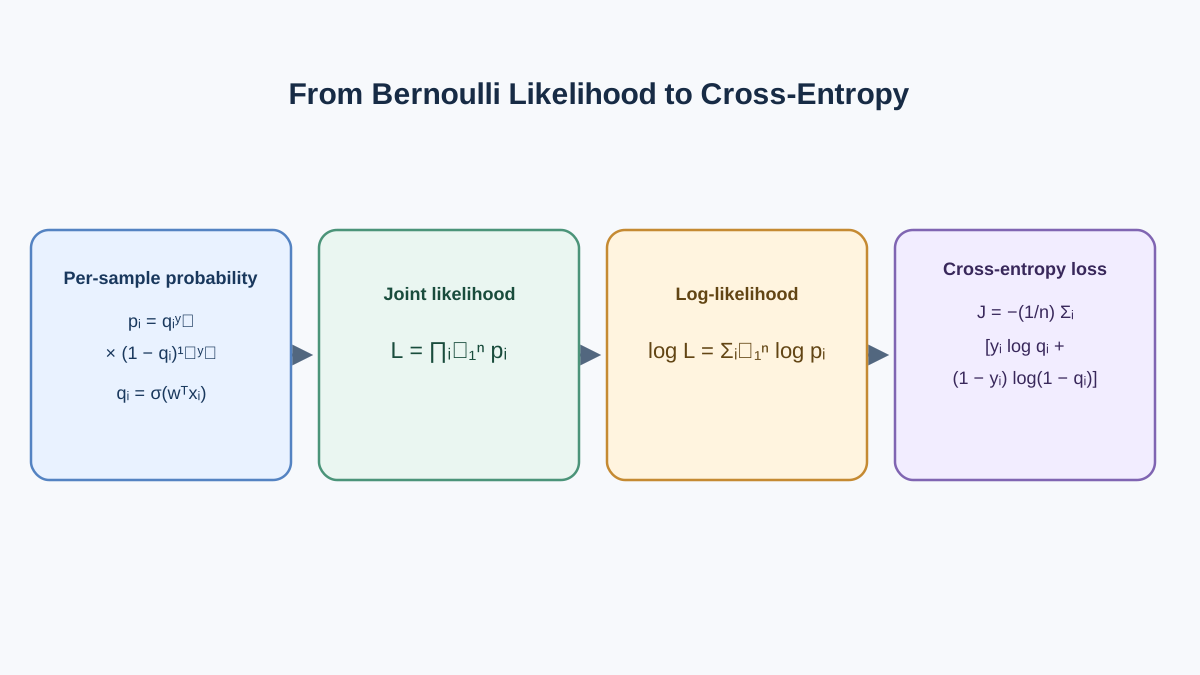
Multiply the per-sample probabilities across all samples. That product is the likelihood of the observed labels:
This is the probability of the data you saw, as a function of the parameters. Maximum likelihood estimation says: pick the parameters that make the observed data most probable.
There is a practical problem. Every factor sits between 0 and 1. Multiply a few hundred of them and the product underflows to zero in floating point. Products are also painful to differentiate.
Take the log. The log is monotonic, so it does not move the maximum — the parameters that maximize are the same ones that maximize . This is the step most tutorials skip, and it is the whole reason the log is not a convenience trick. It is a structural simplification.
The product becomes a sum, and the exponents become multiplicative selectors:
For each sample, exactly one term survives. If the true label is 1, you get . If it is 0, you get . The log-likelihood is just a sum of per-sample log-probabilities.
Knowledge check
Check your understanding
Answer this question before you continue.
Maximizing Likelihood Is Minimizing Cross-Entropy
Optimizers are built to minimize. So negate the log-likelihood and divide by to get an average:
That is the cross-entropy loss, also called log loss. Maximizing likelihood and minimizing negative log-likelihood are the same optimization problem, stated in the direction the optimizer expects. Nothing was added. The sign flipped.
Substitute and you have the loss in terms of the linear score. The sigmoid's derivative cancels cleanly against the log's derivative in the gradient, which is a hint that this pairing is not accidental.
Why not squared error? Suppose the true label is 1 and the model predicts . Squared error gives roughly , a bounded penalty. Cross-entropy gives , and it grows without bound as the prediction approaches 0. Squared error on a sigmoid output also produces a non-convex objective with vanishing gradients for confidently wrong predictions. Cross-entropy stays convex in the parameters and punishes confident mistakes sharply.
Warning: Cross-entropy is the right objective when the model outputs a probability for a binary label. It is not automatically right for ranking or ordinal outcomes, where the target structure is not Bernoulli. Unequal decision costs are a separate issue: they usually change the decision threshold or the training setup, not the likelihood derivation itself.
Knowledge check
Check your understanding
Answer this question before you continue.
Worked Example: One Feature, Two Coefficients
Let's make this concrete with four points and one feature.
| -1 | 0 |
| 0 | 0 |
| 1 | 1 |
| 2 | 1 |
Start with , . Compute , then :
| per-sample loss | ||||
|---|---|---|---|---|
| -1 | 0 | -1 | 0.269 | 0.313 |
| 0 | 0 | 0 | 0.500 | 0.693 |
| 1 | 1 | 1 | 0.731 | 0.313 |
| 2 | 1 | 2 | 0.881 | 0.127 |
The average loss is .
Now nudge up to . The scores spread out, the probabilities sharpen, and the average loss drops to roughly . The loss moved in the direction the derivation predicts: increasing the weight on a feature that separates the classes lowers the negative log-likelihood.
Look at the asymmetry. The sample at with a true label of 1 contributes only because the model is already confident and correct. If the model had predicted for that same label, the term would be — a single sample dominating the sum. That is the behavior the derivation bought us: confident errors are expensive, confident correct answers are nearly free.
You can verify the hand calculation against scikit-learn on the same data. Fit LogisticRegression with regularization disabled and compare the reported loss. The numbers should agree.
Reading the Fitted Parameters
Now the payoff. A fitted coefficient is the change in the log-odds of the positive class per one-unit increase in that feature, holding the others fixed. Log-odds is , and the model is linear in it.
Exponentiate a coefficient and you get an odds ratio — a multiplicative change in odds. An odds ratio of 2 means a one-unit increase doubles the odds. That framing is often easier to hand to a stakeholder than a raw log-odds number.
There is a fast approximation worth knowing. Divide a coefficient by 4 to estimate the largest change in predicted probability a one-unit increase can produce. The maximum slope of the sigmoid is , so this is where the shortcut comes from. It is a rough read, not a precise one.
Common mistake: A coefficient is not a change in probability, and its magnitude is not comparable across features measured on different scales. Standardize before comparing.
One failure mode deserves a flag. When the classes are perfectly separable, the likelihood keeps increasing as the weights grow without bound, so the coefficients diverge. Regularization is the practical fix, and it is why scikit-learn applies it by default.
Knowledge check
Check your understanding
Answer this question before you continue.
What the Derivation Buys You
The loss function is not a library convention. It is the negative log-likelihood of a Bernoulli model, and that is why it behaves the way it does.
The decision rule: when you see a probability output paired with cross-entropy loss, you are looking at a maximum-likelihood fit. When the loss and the output distribution disagree, the model is mismatched to the problem.
This same derivation generalizes. Swap the Bernoulli for a categorical distribution and you get softmax and multiclass cross-entropy. The pattern recurs anywhere a model outputs probabilities.
Your next move: take the gradient of the cross-entropy loss with respect to and and confirm it reduces to . That clean form is what makes gradient descent on logistic regression almost trivial to implement, and deriving it yourself is the natural continuation of everything above.
Knowledge check
Final check
Finish the article by checking the ideas you just learned.
References
Build stronger machine learning foundations
Use structured resources to connect theory, scikit-learn workflows, and evaluation practice.


