
Logistic Regression for Classification: From Scores to Probabilities
A logistic regression prediction is not a label. It is a probability—and the label is a decision you make on top of that probability.

Key topics
A logistic regression prediction is not a label. It is a probability—and the label is a decision you make on top of that probability.
If you have worked with linear regression, the name "logistic regression" probably feels like a contradiction. Regression predicts numbers: house prices, temperatures, revenue. Classification predicts categories: spam or not spam, approved or denied, malignant or benign. So why does a classifier carry the word "regression" in its name?
The answer reveals something useful about how this model actually works. Logistic regression keeps the machinery of linear regression—the weighted sum of features—but changes what that sum means and how the model learns. Understanding that shift is the difference between treating logistic regression as a black box and being able to read its predictions with confidence.
Why "Regression" Is in the Name of a Classifier
Linear regression computes a weighted sum of your features plus an intercept, then uses that sum directly as its prediction. If you are predicting a house price, the model might output $412,000. If you are predicting temperature, it might output 23.5°C. The output is unbounded—it can be any real number.
Logistic regression starts with the exact same calculation. It still multiplies each feature by a learned weight, adds them together, and adds an intercept. That part is pure linear regression. What changes is what happens next.
Instead of treating that weighted sum as the final answer, logistic regression passes it through a transformation that forces the output into the range between 0 and 1. The result is a probability: the chance that an example belongs to the positive class.
So the name survives because the mechanism is a linear model. The output layer and the loss function are what make it a classifier. Linear regression predicts an unbounded number; logistic regression predicts a probability bounded between 0 and 1.
That raises the central question this article answers: how does a linear score become a probability, and how does that probability become a decision?
Knowledge check
Check your understanding
Answer this question before you continue.
The Logit: A Linear Score With No Natural Bounds
Before the transformation, logistic regression produces something called a logit—a raw score computed exactly like a linear regression prediction:
logit = weight_1 * feature_1 + weight_2 * feature_2 + ... + intercept
If you have seen linear regression, this shape is familiar. Each feature contributes to the score according to its learned weight. A positive weight pushes the score up; a negative weight pushes it down.
The problem is that this score has no natural bounds. Feed it a very large feature value and the logit can climb to 50 or 500. Feed it a very small one and it can drop to -50 or -500. That is fine when you are predicting a continuous quantity, but it is awkward for classification. A probability must stay between 0 and 1. A score of 37 is not a probability of anything.
The logit does have an intuitive meaning, though. It represents the log-odds of the positive class—a measure of how much evidence points toward class 1 versus class 0. A logit of 0 means the evidence is perfectly balanced. A large positive logit means strong evidence for the positive class. A large negative logit means strong evidence against it.
Think of a spam filter. Suppose the model uses the number of suspicious phrases in an email as a feature. An email with zero suspicious phrases might produce a logit of -4.2. An email packed with them might produce a logit of 3.8. Both are legitimate scores, but neither can be read directly as a probability. The score needs to be squeezed into the 0-to-1 range first.
Knowledge check
Check your understanding
Answer this question before you continue.
The Sigmoid: Squeezing a Score Into a Probability
The transformation that does the squeezing is called the sigmoid function, also known as the logistic function. It takes any real number and maps it to a value between 0 and 1.
The sigmoid has a distinctive S-shape. Large positive logits get pushed close to 1 but never quite reach it. Large negative logits get pushed close to 0 but never quite reach it. A logit of exactly 0 maps to 0.5—perfect uncertainty.
Here is what the mapping looks like for a few logit values:
| Logit | Sigmoid output (probability) |
|---|---|
| -5 | 0.007 |
| -2 | 0.12 |
| 0 | 0.50 |
| 2 | 0.88 |
| 5 | 0.993 |
Notice what the sigmoid does that a straight line cannot. A linear transformation of the score would eventually produce values below 0 or above 1 as the score grows. The sigmoid compresses those extremes so the output always stays in the valid probability range.
This is also where the analogy to linear regression stops being exact. In linear regression, the relationship between features and the prediction is linear: increase a feature by one unit and the prediction changes by a fixed amount. In logistic regression, the relationship between features and the probability is curved. Increasing a feature by one unit changes the logit by a fixed amount, but the effect on the probability depends on where you start. Moving from a logit of 0 to 1 shifts the probability from 0.50 to 0.73. Moving from a logit of 3 to 4 shifts it only from 0.95 to 0.98. The same feature change matters less when the model is already confident.
If you plot the sigmoid curve and mark a few logit values along the horizontal axis, you can see this directly: the curve is steepest near 0 and flattens out at both ends. That shape is why the sigmoid is well suited to probabilities. It reserves the model's sensitivity for the region where the evidence is genuinely ambiguous.
Knowledge check
Check your understanding
Answer this question before you continue.
From Probability to Decision: The Threshold Is a Choice
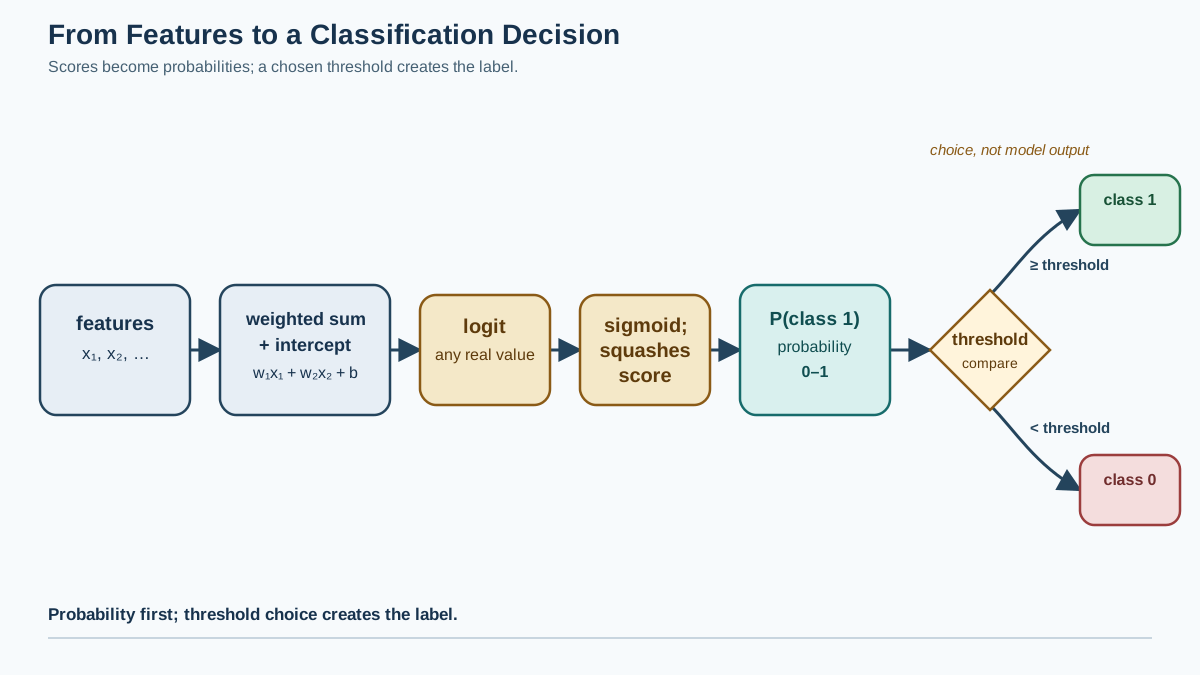
Once the model outputs a probability, you still need a class label. Spam filters do not report "72% spam"—they move the email to the spam folder or they do not. That step from probability to label is where the threshold comes in.
The default threshold is 0.5: predict the positive class when the probability is at or above 0.5, and the negative class otherwise. This is a reasonable starting point, but it is not a law of mathematics. It is a choice, and it is only the right choice when the two classes are equally costly to get wrong.
Consider the difference between two scenarios.
In spam filtering, a false positive—a legitimate email marked as spam—can mean a missed message from a client or an employer. A false negative, by contrast, just leaves one unwanted email in your inbox. The costs are not symmetric. If missing an important email is expensive, you might lower the threshold to 0.3, accepting more spam in the inbox to reduce the chance of losing a real message.
In disease screening, the tradeoff flips. Missing a positive case can be life-threatening, while a false alarm usually leads to a follow-up test. A screening model might use a threshold of 0.1 or even lower, accepting many false positives to catch nearly every true case.
Moving the threshold trades off false positives against false negatives. Raise the threshold and the model becomes more conservative—fewer positive predictions, but the ones it makes are more likely to be correct. Lower the threshold and the model becomes more aggressive—more positive predictions, including more mistakes.
My rule is simple: choose the threshold by the cost of each error type, not by convention. If you are not sure which error is more expensive, start at 0.5 and then deliberately test what happens as you move it.
There is also a deeper point here. The probability itself is often more useful than the label. When you are ranking customers by risk or prioritizing which support tickets to handle first, the raw probability gives you an ordering that a binary label destroys. A 51% probability and a 99% probability both become "positive" at a 0.5 threshold, but they are very different predictions. The probability is the model's real output; the label is a decision you impose on it.
Note: When you tune a threshold, do it on validation data, not the test set. Fit the model on training data, evaluate candidate thresholds on validation data using your error costs or a target metric, then run the final evaluation once on held-out test data. Tuning the threshold on test data makes your reported performance optimistic.
Knowledge check
Check your understanding
Answer this question before you continue.
How the Model Learns: Cross-Entropy Loss
Training a logistic regression model means finding the weights that produce good probabilities. But "good" needs a precise definition, and the definition matters more than you might expect.
You might wonder why logistic regression does not simply minimize squared error, the way linear regression does. After all, if the goal is to get probabilities close to the true labels (0 or 1), squared error seems like a natural measure of closeness.
The problem is that squared error was designed for continuous targets, not for probabilities. It treats the gap between a prediction and the label as if it were a distance along a number line. But a probability is not just a number to be approximated—it is a statement about how likely each outcome is. When the true label is 1, a prediction of 0.99 and a prediction of 0.51 are both "correct" in the sense that they round to the right class. But they are not equally good probabilistic statements. The first says the positive class is nearly certain; the second says it is barely more likely than not.
Logistic regression uses a different loss function called cross-entropy loss, also known as log loss. Cross-entropy measures how well the predicted probability distribution matches the actual outcome. When the true class is 1, the loss grows without bound as the predicted probability of class 1 approaches 0. A prediction of 0.01 for a true positive case is not just a miss—it is a catastrophic miss, because the model assigned almost no probability to the event that actually happened.
Here is the key contrast. For a true label of 1:
- Squared error for a prediction of 0.99: (1 - 0.99)² = 0.0001
- Squared error for a prediction of 0.51: (1 - 0.51)² = 0.2401
- Squared error for a prediction of 0.01: (1 - 0.01)² = 0.9801
Squared error does penalize the confidently wrong prediction more, but the penalty grows only quadratically. Cross-entropy grows much faster as the predicted probability approaches 0. The difference matters during training: cross-entropy gives the optimizer a much stronger gradient signal to pull the model away from confidently wrong predictions.
This is not a mathematical detail. The choice of loss function shapes what the model learns to do. Cross-entropy rewards the model for assigning high probability to the observed class and punishes it severely for assigning near-zero probability to what actually happened. That is exactly the behavior you want from a probabilistic classifier.
Common mistake: Do not assume cross-entropy automatically produces calibrated probabilities. The loss trains the model to be probabilistically honest, but calibration—whether a predicted 0.8 really means the event happens about 80% of the time—depends on your data, features, and model fit. If probabilities drive decisions, check calibration on validation data rather than assuming it.
When Logistic Regression Fits—and When It Does Not
Logistic regression is not the right tool for every classification problem. Knowing where it shines and where it struggles is part of understanding what it actually is.
The strengths are substantial. Logistic regression produces natural probabilities that are often well-calibrated when the model fits the data well—a predicted probability of 0.8 means the event happens about 80% of the time. The coefficients are interpretable: you can inspect the weight for each feature and understand its direction and rough magnitude of influence. The model trains quickly, even on large datasets, and performs well with modest amounts of data. When your decision boundary is roughly linear in log-odds space, logistic regression is hard to beat.
The limitations are equally real. Logistic regression assumes a roughly linear relationship between features and the log-odds of the positive class. If the true boundary is highly nonlinear—say, a circular region of positive examples surrounded by negatives—a plain logistic regression model will struggle. Interactions between features must be added manually. If the effect of one feature depends on the value of another, the model will not discover that on its own.
In practice, I treat logistic regression as the first model I try for most binary classification problems. It gives me a baseline, interpretable coefficients, and probabilities I can inspect. If a tree-based model beats it by a wide margin on validation data, that gap is information: it tells me the decision boundary is probably nonlinear, and I can decide whether the extra complexity is worth it.
When interpretability or trustworthy probabilities matter more than squeezing out the last accuracy point, logistic regression is often the right choice even when a more complex model could score slightly higher. A model you can explain to a stakeholder or a regulator has value that does not show up in an accuracy metric.
The full chain should now be clear. The model computes a linear score—the logit—that measures evidence for the positive class. The sigmoid squeezes that score into a probability between 0 and 1. Cross-entropy loss trains the model to assign high probability to the observed class. And the threshold, which you choose based on the cost of errors, converts the probability into a decision.
The next time you fit a logistic regression model, do not just read the predicted labels. Inspect the raw probabilities. Look at the distribution of predictions for each class. Try moving the threshold on validation data and watch how the confusion matrix changes. That exercise will teach you more about your problem—and about what logistic regression classification actually does—than any default setting ever will.
Knowledge check
Final check
Finish the article by checking the ideas you just learned.
References
Research updated Sep 8, 2026


