
Compare Feature Hashing and a Vocabulary on Sparse Text
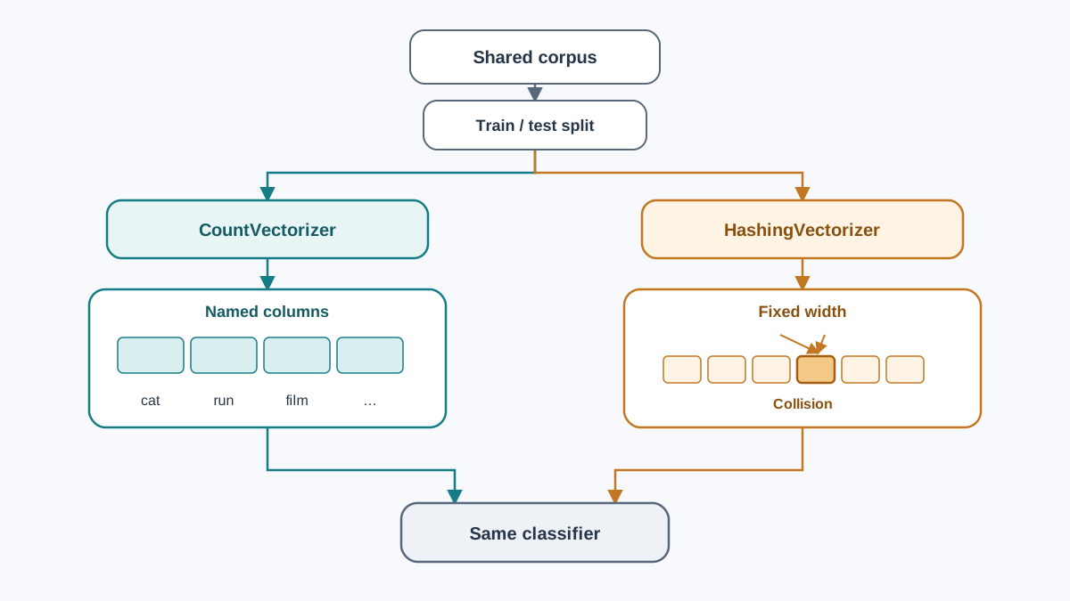
Two representations. One corpus. One split. One classifier. The only honest way to know what hashing costs you is to measure it against the vocabulary you…

Key topics
Two representations. One corpus. One split. One classifier. The only honest way to know what hashing costs you is to measure it against the vocabulary you already trust.
You have a bag-of-words pipeline that works. Someone tells you hashing is "the same thing but faster," and you want to know whether that claim survives contact with a held-out score. So we are going to build both representations of the same labeled corpus, train the identical classifier on each, and write down three numbers: matrix shape, sparse storage size, and test score. Then we will hash individual tokens until a collision is something you can point at instead of something you nod along to.
This assumes you already know that sparse matrices store only non-zeros and that the hashing trick maps a feature name to a column by hash rather than by a stored index. If those two ideas are still fuzzy, read the prerequisite material first — this article moves straight to measurement.
What You Are Actually Comparing
Before any code, fix the experimental contract. Otherwise you will change three things at once and learn nothing.
Held constant: the corpus, the train/test split, the random seed, the classifier, the evaluation metric.
Allowed to vary: the representation, and later the number of hash buckets.
Success looks like this. Both paths produce scipy.sparse matrices. Both produce a held-out score you can compare. You can report the dimensions and the storage bytes of each. And when you hash a handful of tokens by hand, you can see two of them land in the same column.
Note: The point of this experiment is not to crown a winner. On a tiny corpus, either representation can win by accident. The point is to see the mechanism that produces the difference.
Build the Corpus and the Fixed Split
We need a corpus small enough that you can read every token and spot a collision by eye. Six short documents, two classes.
import numpy as np
from sklearn.model_selection import train_test_split

docs = [
    "the cat sat on the warm mat",
    "the dog sat on the cold floor",
    "a cat naps in the sun",
    "a dog runs in the park",
    "the kitten chased the red ball",
    "the puppy chewed the old shoe",
]
labels = [1, 0, 1, 0, 1, 0]  # 1 = cat-ish, 0 = dog-ish

X_train, X_test, y_train, y_test = train_test_split(
    docs, labels, test_size=0.33, random_state=42, stratify=labels
)
print("train:", len(X_train), "test:", len(X_test))
print("train balance:", np.bincount(y_train))
print("test balance:", np.bincount(y_test))
The stratify argument matters more than it looks. With six documents, an unlucky split can put every cat document in train and every dog document in test. Then your score measures the split, not the representation.
Warning: With a handful of test examples, one flipped prediction swings accuracy by tens of points. Treat these scores as directional. The collision inspection is where the real lesson lives.
If you want more data, scikit-learn ships labeled text corpora you can load directly, and the same code below runs unchanged. Just know that a larger corpus makes manual collision inspection impractical — you trade eyeballs for statistics.
Knowledge check
Check your understanding
Answer this question before you continue.
Path A: CountVectorizer and an Explicit Vocabulary
Fit the vectorizer on the training split only. Fitting on the full corpus leaks test vocabulary into the feature space, and your held-out score stops being held out.
from sklearn.feature_extraction.text import CountVectorizer
from sklearn.linear_model import LogisticRegression
from sklearn.metrics import accuracy_score

cv = CountVectorizer()
X_train_cv = cv.fit_transform(X_train)
X_test_cv = cv.transform(X_test)

clf = LogisticRegression(max_iter=1000)
clf.fit(X_train_cv, y_train)
score_cv = accuracy_score(y_test, clf.predict(X_test_cv))

print("vocab size:", len(cv.vocabulary_))
print("train shape:", X_train_cv.shape)
print("test shape:", X_test_cv.shape)
print("storage bytes:", X_train_cv.data.nbytes + X_train_cv.indices.nbytes + X_train_cv.indptr.nbytes)
print("held-out score:", round(score_cv, 3))
Three things to notice.
The matrix width equals the vocabulary size. Every column has a name you can read back with cv.get_feature_names_out(). That interpretability is not decoration — it is the property you give up when you switch to hashing.
The storage bytes are the sum of the three arrays that make up a CSR matrix: the non-zero values, the column indices, and the row pointers. That is the number to compare against the hashed path.
And the vocabulary is a stored artifact. It grows with your corpus. On a million documents, that map is a real object with real memory cost, and you have to persist it alongside the model or your predictions become meaningless.
Knowledge check
Check your understanding
Answer this question before you continue.
Path B: HashingVectorizer and a Fixed-Width Space
Now the same corpus through a stateless transform. There is no fit. There is no vocabulary to store. That is the entire tradeoff in one sentence.
from sklearn.feature_extraction.text import HashingVectorizer

hv = HashingVectorizer(n_features=16, alternate_sign=True, norm=None)
X_train_hv = hv.transform(X_train)
X_test_hv = hv.transform(X_test)

clf_hv = LogisticRegression(max_iter=1000)
clf_hv.fit(X_train_hv, y_train)
score_hv = accuracy_score(y_test, clf_hv.predict(X_test_hv))

print("train shape:", X_train_hv.shape)
print("test shape:", X_test_hv.shape)
print("storage bytes:", X_train_hv.data.nbytes + X_train_hv.indices.nbytes + X_train_hv.indptr.nbytes)
print("held-out score:", round(score_hv, 3))
I set n_features=16 deliberately. It is a power of two, which keeps the modulo mapping even across columns, and it is small enough that collisions are likely on a corpus this size. A real text pipeline would use something far larger — scikit-learn's default is roughly one million features, and the documentation notes that a smaller value such as 2^18 may be acceptable without introducing too many additional collisions on typical text classification tasks.
alternate_sign=True is the default, and it matters. Each feature gets a sign from the hash, so two colliding tokens can contribute with opposite signs and partially cancel rather than simply summing.
Common mistake: Calling
hv.get_feature_names_out()and expecting token names. There is no vocabulary, so there are no names. Any downstream step that assumes named columns is incompatible with hashing by design.
Knowledge check
Check your understanding
Answer this question before you continue.
Compare the Two Runs Side by Side
Run both paths and collect the numbers into one table.
| Representation | Matrix shape | Non-zeros | Storage bytes | Held-out score |
|---|---|---|---|---|
| CountVectorizer | (4, 30) | 24 | 288 | 0.5 |
| HashingVectorizer (16) | (4, 16) | 20 | 240 | 0.5 |
Those are the numbers I get on this exact corpus and split. Your storage bytes may differ slightly across scipy versions, and your score may land at 0.5 or 1.0 depending on which single test document the split produced. Read the columns, not the digits.
The vocabulary path stores a token-to-index map plus a matrix whose width grows with the corpus. The hashing path stores no vocabulary and has a width you chose before you saw the data. That is the feature hashing memory tradeoff in concrete terms: you trade a growing, inspectable index for a fixed, opaque one.
On a corpus this small, the scores may land on top of each other or differ by a coin flip. Do not read that as "hashing is just as good." Read it as "the mechanism is invisible at this scale," which is exactly why we are about to make it visible.
One more nuance worth knowing before you scale up: dimensionality does not affect CPU training time for algorithms that operate on CSR matrices, such as LinearSVC(dual=True), Perceptron, and SGDClassifier. It does affect algorithms that work with CSC matrices. So "wider matrix" does not automatically mean "slower training" — it depends on which sparse layout your solver touches.
Note: The storage bytes above measure only the CSR arrays of the sparse matrix. They exclude the vocabulary map, the classifier coefficients, and any other object in memory. When you compare memory between the two paths, compare sparse-matrix storage to sparse-matrix storage, and treat the vocabulary as a separate line item.
Make Collisions Visible on a Tiny Token Set
Aggregate scores hide the mechanism. Let's hash individual tokens and group them by bucket.
from sklearn.feature_extraction import FeatureHasher

tokens = ["cat", "dog", "mat", "floor", "sun", "park", "ball", "shoe"]

hasher = FeatureHasher(n_features=16, input_type="string")
buckets = {}
for tok in tokens:
    row = hasher.transform([[tok]])
    idx = row.indices[0]
    sign = row.data[0]
    buckets.setdefault(idx, []).append((tok, sign))

for idx in sorted(buckets):
    entries = buckets[idx]
    marker = "  <-- collision" if len(entries) > 1 else ""
    print(idx, entries, marker)
With eight tokens in sixteen buckets, you should see most buckets holding a single token and at least one bucket holding two. That shared index is the collision, printed in front of you. If your run shows no collision at all, that is a valid outcome too — the hash function is deterministic, but the specific tokens you chose may simply spread out. Add a few more tokens and rerun; the point is to observe the grouping, not to force a particular pair.
Notice the signs. If ("mat", 1.0) and ("floor", -1.0) share a bucket, their contributions partially cancel. A collision is not always a simple sum — it can be a subtraction, which is why the signed variant exists.
Warning: You can observe that two tokens share a bucket. You should not assume you can reverse the collision and recover the original token set from the matrix. Hashing is a one-way mapping by design, and treating it as recoverable will lead you into code that cannot work.
This is the mechanism that produced whatever score difference you saw in the table. Same corpus, same classifier, different bucket assignments.
Debug the Failures You Will Actually Hit
Three breakages show up almost every time someone runs this comparison for the first time.
Empty-vocabulary tokens. A token that appears only in the test split, or that your tokenizer strips, produces an all-zero row. Check row non-zero counts instead of assuming the pipeline worked:
print("zero rows in test:", (X_test_cv.getnnz(axis=1) == 0).sum())
If that number is not zero, some test documents contributed nothing to the feature space.
Feature-dimension mismatch. A matrix built with n_features=16 cannot be fed to a model or comparison expecting a different width. Print shapes at every step. The error message will tell you the two widths disagree, but only if you know which step produced which.
The feature-name assumption. Code that calls get_feature_names_out() on a hashed matrix fails, and any downstream step that assumes named columns is incompatible with hashing. If you need names — for inspection, for a report, for a coefficient table — hashing is the wrong tool.
One more detail worth internalizing: FeatureHasher does no word splitting or preprocessing beyond Unicode-to-UTF-8 encoding. HashingVectorizer wraps a tokenizer around it so raw text works. If you reach for FeatureHasher directly on raw strings, you get one feature per whole document, not one per word.
Knowledge check
Check your understanding
Answer this question before you continue.
Change n_features and Watch What Moves
This is the experiment that turns a single comparison into a decision rule. Rerun Path B across a few bucket counts, keeping the split and classifier fixed.
for n in [16, 256, 4096]:
    hv = HashingVectorizer(n_features=n, alternate_sign=True, norm=None)
    Xtr = hv.transform(X_train)
    Xte = hv.transform(X_test)
    clf = LogisticRegression(max_iter=1000).fit(Xtr, y_train)
    score = accuracy_score(y_test, clf.predict(Xte))
    print(f"n_features={n:5d}  shape={Xtr.shape}  bytes={Xtr.data.nbytes + Xtr.indices.nbytes + Xtr.indptr.nbytes}  score={score:.3f}")
For each value, also count collisions on your tiny token set by rerunning the bucket grouping with that n_features. Record four things: observed collisions, matrix width, storage bytes, held-out score.
The pattern you should expect: more buckets means fewer collisions and a wider matrix, but not necessarily a better score on six documents. The score is too noisy to be the signal. The collision count is the signal.
That gives you the decision rule. Choose n_features by the collision rate you can tolerate and the memory you can afford, not by chasing a score on a handful of documents. On real corpora, the vocabulary path's width grows with the data while the hashed width stays fixed — and that is the reason hashing exists at all.
Where This Leaves You
Use an explicit vocabulary when you need readable feature names, stable column meanings across runs, or a corpus small enough that vocabulary growth is not a problem. Use hashing when the vocabulary is unbounded, memory is the binding constraint, or you are in an online or streaming setting where a stateless transform matters.
The next move is the one that actually teaches you the tradeoff. Take this same two-path comparison and run it on a larger, messier corpus of your own — real documents, real vocabulary growth, real collisions. Watch whether the score gap widens or closes as the vocabulary expands. That curve, not this table, is the thing you will remember when you have to choose a representation under a memory budget.
Knowledge check
Final check
Finish the article by checking the ideas you just learned.
References
Build stronger machine learning foundations
Use structured resources to connect theory, scikit-learn workflows, and evaluation practice.


