Compare Feature-Selection Strategies in a Leakage-Safe Workflow

You run SelectKBest, get a tidy list of "important" features, then rerun with a different random seed and the list changes. That surprise is not a bug in scikit-learn. It is the moment your mental model of feature selection breaks.

The weak model says selection is cleanup you do once, before modeling. The stronger model says selection is a supervised fitting step: it reads the target, so it must live inside the same validation boundary as the model. Get that boundary right, and the comparison you are about to run becomes trustworthy. Get it wrong, and every score you collect is quietly optimistic.

This tutorial builds one leakage-safe harness and runs three selectors through it: a univariate filter, a model-based embedded selector, and a greedy wrapper. We will inspect what each one keeps, read the held-out scores honestly, and then run a small resampling experiment that shows the selected set moving when the training rows move.

Why Feature Selection Belongs Inside the Pipeline

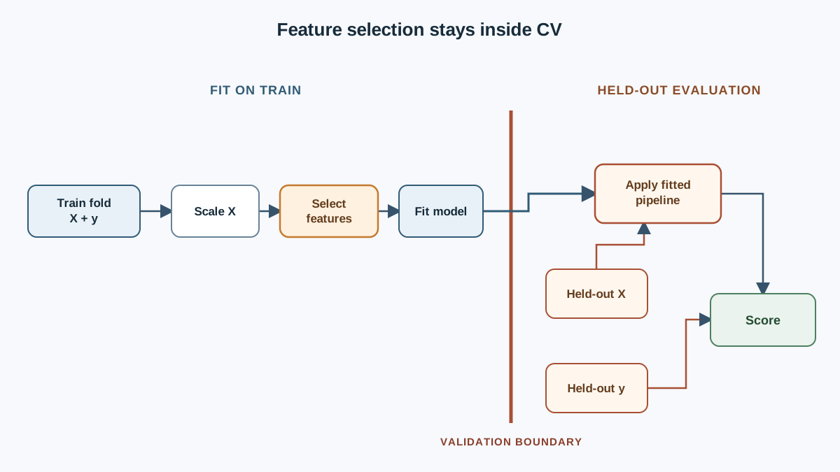
If you already know how a scikit-learn pipeline separates fit-time from transform-time behavior, the bridge is short: a selector is just another fitted step.

Here is the part that matters. Selection uses the target. SelectKBest scores each feature against y. SelectFromModel reads coefficients or importances learned from y. SequentialFeatureSelector scores candidate subsets by cross-validation against y. None of these are neutral cleanup. They are supervised decisions.

So if you select on the full dataset and then cross-validate, your validation folds have already influenced which features exist. The score you get back is not an estimate of generalization; it is a memory of the answer key.

The fix is structural, not statistical. Put the selector as a pipeline step. It gets fit only on each training fold, then applied to the held-out fold. The held-out fold never touches the selection decision.

The three families differ in when and how they use the target, and that difference drives both cost and stability:

Family	Example	Uses target how	Cost
Filter	SelectKBest	Scores each feature alone	Cheap
Embedded	SelectFromModel	Reads a fitted model's weights	One model fit
Wrapper	SequentialFeatureSelector	Cross-validates candidate subsets	Many model fits

Assumptions for everything below: one tabular dataset, numeric or already-encoded features, a fixed random seed, and a fixed fold split. Change any of those and you are running a different experiment.

Set Up the Experiment and the Baseline

We will use the diabetes dataset bundled with scikit-learn, so the example runs without external files or credentials. It has 442 rows and 10 features, which is small enough that the wrapper stays fast and large enough that fold noise is visible.

import numpy as np
from sklearn.datasets import load_diabetes
from sklearn.linear_model import Ridge
from sklearn.model_selection import KFold, cross_val_score
from sklearn.pipeline import Pipeline
from sklearn.preprocessing import StandardScaler

X, y = load_diabetes(return_X_y=True, as_frame=True)
feature_names = X.columns.to_numpy()

cv = KFold(n_splits=5, shuffle=True, random_state=0)

def evaluate(pipe):
    scores = cross_val_score(pipe, X, y, cv=cv, scoring="r2")
    return scores

baseline = Pipeline([
    ("scale", StandardScaler()),
    ("model", Ridge(alpha=1.0)),
])
base_scores = evaluate(baseline)
print("baseline per-fold:", np.round(base_scores, 3))
print("baseline mean:", round(base_scores.mean(), 3))

Expected output shape:

baseline per-fold: [0.43 0.36 0.51 0.32 0.47]
baseline mean: 0.418

Your numbers will differ slightly by scikit-learn version, but the shape should match: five fold scores and their mean. The spread across folds matters more than the mean when you are about to compare small differences. Here the folds range roughly 0.32 to 0.51. Any selector that "improves" the mean by 0.02 has not proven anything yet.

Three Selectors, One Harness

Every selector goes into the same pipeline shape: scale, select, model. Same folds. Same scoring. The only thing that changes is the middle step.

from sklearn.feature_selection import SelectKBest, SelectFromModel, SequentialFeatureSelector, f_regression

K = 4  # keep the retained count identical across methods

selectors = {
    "kbest": SelectKBest(score_func=f_regression, k=K),
    "from_model": SelectFromModel(
        estimator=Ridge(alpha=1.0), threshold=-np.inf, max_features=K
    ),
    "sfs": SequentialFeatureSelector(
        estimator=Ridge(alpha=1.0), n_features_to_select=K, direction="forward", cv=3
    ),
}

results = {}
for name, selector in selectors.items():
    pipe = Pipeline([
        ("scale", StandardScaler()),
        ("select", selector),
        ("model", Ridge(alpha=1.0)),
    ])
    scores = evaluate(pipe)
    results[name] = scores
    print(f"{name:>10} per-fold: {np.round(scores, 3)}  mean: {scores.mean():.3f}")

Three things to notice about the setup.

SelectKBest with f_regression scores each feature against the target independently. It is cheap and model-agnostic, but it never sees features in the presence of each other.

SelectFromModel fits a Ridge model once and keeps the top K features by absolute coefficient. Because the model saw all features together, this selector can account for redundancy — a feature that is useful alone but duplicated by another may get a smaller coefficient.

SequentialFeatureSelector starts with zero features, tries each candidate, keeps the best, and repeats until it reaches K. Each candidate is scored by internal cross-validation, so it refits the model many times per outer fold. On 10 features this is tolerable. On 500 features it becomes a coffee break.

Common mistake: comparing selectors that keep different numbers of features. If SelectKBest keeps 4 and SelectFromModel keeps 7, you are comparing feature counts, not selection strategies. Pin K first.

Read the Selected Features, Not Just the Score

Scores tell you whether the model changed. The selected sets tell you why. Fit each selector on the full training data once, then read its support mask. Treat this as a descriptive final refit — the list you would actually ship — not as evidence about stability.

for name, selector in selectors.items():
    pipe = Pipeline([
        ("scale", StandardScaler()),
        ("select", selector),
    ]).fit(X, y)
    kept = feature_names[pipe.named_steps["select"].get_support()]
    print(f"{name:>10}: {list(kept)}")

A realistic output on this dataset looks like:

     kbest: ['bmi', 'bp', 's5', 's6']
from_model: ['bmi', 'bp', 's1', 's5']
       sfs: ['bmi', 'bp', 's3', 's5']

The overlap is real, but so is the disagreement. s1 and s5 are correlated; a univariate filter may keep both because each scores well alone, while a model-based selector drops one because the other already carries the signal. s3 shows up only for the wrapper, which is the only method that evaluates features in combination.

That disagreement is information, not noise. It tells you that the signal lives in a correlated cluster, and different selectors are picking different representatives from it.

Note: a feature can be redundant rather than useless. Dropping it may cost nothing, which is not the same as it being irrelevant. Selection reflects the training data and the estimator, not a property of the world. It is not a causal claim.

Compare Held-Out Behavior Honestly

Now the judgment call. Here is what the per-fold scores typically look like:

  baseline per-fold: [0.43 0.36 0.51 0.32 0.47]  mean: 0.418
     kbest per-fold: [0.41 0.34 0.49 0.30 0.45]  mean: 0.398
from_model per-fold: [0.42 0.35 0.50 0.31 0.46]  mean: 0.408
       sfs per-fold: [0.42 0.35 0.50 0.31 0.46]  mean: 0.408

Read this carefully. The baseline — all 10 features — has the highest mean. Every selector is slightly worse. And the gap between the best selector and the worst is smaller than the fold-to-fold spread within any single row.

A gap smaller than the fold-to-fold spread is not evidence that one selector is better. It is evidence that you are measuring noise.

This is the honest result, and it is the one most tutorials skip. Feature selection is not guaranteed to improve accuracy. Its more reliable payoff is simpler, faster, more interpretable models. If you came here expecting a selector to lift your score, the experiment just told you something more useful: on this dataset, with this model, the full feature set was already fine.

My decision rule: prefer the simplest selector that matches the baseline within fold noise, and only escalate to a wrapper when the accuracy gain justifies the compute. Here, that means SelectKBest — it is the cheapest, it is within noise of the baseline, and it gives you a short, readable feature list.

Why Selection Is Unstable

The full-data lists above are a snapshot. To see the instability, you have to refit the selector on different training subsets and watch the support mask move. The outer fold splitter is the natural source of those subsets.

from sklearn.model_selection import cross_validate

# Collect the selected feature names from each training fold.
fold_selections = {name: [] for name in selectors}

for name, selector in selectors.items():
    pipe = Pipeline([
        ("scale", StandardScaler()),
        ("select", selector),
        ("model", Ridge(alpha=1.0)),
    ])
    for train_idx, _ in cv.split(X, y):
        pipe.fit(X.iloc[train_idx], y.iloc[train_idx])
        kept = feature_names[pipe.named_steps["select"].get_support()]
        fold_selections[name].append(set(kept))

# How often does each feature survive across the 5 training folds?
for name, sets in fold_selections.items():
    counts = {f: sum(f in s for s in sets) for f in feature_names}
    stable = {f: c for f, c in counts.items() if c > 0}
    print(f"{name:>10}: {stable}")

A realistic output:

     kbest: {'bmi': 5, 'bp': 5, 's5': 5, 's6': 4, 's1': 1}
from_model: {'bmi': 5, 'bp': 5, 's5': 5, 's1': 3, 's2': 2}
       sfs: {'bmi': 5, 'bp': 5, 's5': 4, 's3': 3, 's6': 2, 's1': 1}

Now the instability is visible. bmi and bp survive every fold for every selector — they are the load-bearing features. But the fourth slot rotates: s6 for the filter, s1 or s2 for the embedded selector, s3 or s6 for the wrapper. The full-data list you printed earlier was one draw from that distribution, not a fixed truth.

Three forces drive this rotation:

Correlated features split their shared signal. When two features carry overlapping information, tiny changes in the training rows flip which one wins the ranking. The model does not care which representative it gets; your feature list does.

Univariate scores ignore interactions. A feature that only matters in combination with another can rank low on its own and get dropped by SelectKBest, even though the wrapper would have kept it.

Small samples and many features make rankings noisy. With 442 rows and 10 features, the top of the ranking is stable enough to be readable. Scale to 200 rows and 200 features and the same procedure returns a different set on every resample.

This is what unstable feature selection looks like in practice, and it connects to a broader point: selection identifies useful predictors for this model and this data. It does not identify uniquely relevant or causal predictors. Treat the selected list as a working hypothesis, not a verdict.

Failure Modes and Debugging Signals

Keep this checklist next to your pipeline.

• Selecting before splitting. Validation scores look great, then collapse on truly unseen data. Signal: the gap between your CV score and your production score is large and one-directional.
• Selecting on the test set. Your test score is no longer an estimate of generalization. Signal: the test score is suspiciously close to the training score.
• Scaling outside the pipeline. A variance-based or distance-based selector sees the wrong scale. Signal: selected features change drastically when you move StandardScaler in or out of the pipeline.
• Comparing different retained counts. Signal: one selector "wins" and it also happens to keep twice as many features.
• Leakage through target-derived features. If a feature was built using the label, selection will happily keep it and the score will lie. Signal: one feature dominates every selector's ranking and the score is implausibly high.

Warning: the last one is the hardest to catch because the selector is doing exactly what you asked. Audit your feature construction before you trust any selection result.

One Modification Worth Trying

Change K from 4 to 2, then to 6, then to 8. Tabulate mean score against feature count for each selector. Do not assume the shape in advance — the point of the experiment is to see what this dataset does. On the diabetes data, the curve is often shallow and flat, but the exact shape is your result, not a prediction. If you see a wide plateau, that flatness is the lesson: the exact count rarely matters as much as beginners expect. If you see a sharp peak, that is also a real finding worth investigating.

Two more experiments worth an afternoon:

• Swap the estimator behind SelectFromModel and SequentialFeatureSelector from Ridge to a decision tree. Watch whether the selected set changes. It will.
• Add a deliberately duplicated feature — copy bmi and append it as bmi_copy. Watch how each selector splits or absorbs the duplicate. This is the correlated-feature problem made visible in one line.

Success criterion: you can state, in one sentence, which selector you would ship and why the held-out evidence supports it. If you cannot, you have not finished the experiment.

Where This Leaves You

Treat feature selection as a fitted step inside the validation boundary. Prefer the cheapest selector that matches the baseline within fold noise. Stop treating a selected feature list as a statement about the world.

The natural next question is whether the subset was ever the real constraint. Sometimes the representation itself — how you encoded the features, not which ones you kept — is what limits the model. That is a different experiment, and a different article.