Sparse Data in Machine Learning: Many Possible Features, Few Present

You one-hot encoded a categorical column and watched it explode into hundreds of columns. Now your dataset is mostly zeros—and your first instinct might be to clean up all that "wasted space."

Don't. Those zeros are information, and the structure they create is an asset worth protecting.

What Makes a Feature Matrix Sparse

A sparse feature matrix is one where most entries are zero. Not missing. Not unknown. Present-but-zero.

Here's the distinction that trips up nearly every beginner: sparse data is different from missing data.

• Missing data means a value was never recorded. The cell is empty, unknown, or absent. You might impute it, drop it, or flag it.
• Sparse data means the value is genuinely zero. The cell is full of meaning: "this category does not apply," "this word did not appear," "this product was not purchased."

Consider one-hot encoding, which you've seen with categorical features. If you encode a product_category column with 300 possible categories, every row becomes a vector of 300 values—exactly one of them a 1, the other 299 all 0. That row is 99.7% zeros, yet it carries complete information. Nothing is missing.

Text data behaves the same way. Count how often each word appears across a set of documents, and you get a matrix where most cells are zero because most documents never use most words.

Common mistake: Treating zeros as gaps to fill. A zero in a one-hot encoded matrix means "this row does not belong to this category." Imputing that zero would invent a category membership that does not exist.

Three Questions to Ask About Your Zeros

Before you decide what to do with a sparse matrix, separate three questions that beginners often mash together:

1. What does zero mean? Is it a genuine absence—"this category does not apply"—or an unknown value that was never recorded? This is a question about your data's meaning.
2. How are the zeros stored? Does your matrix physically record every cell, or does it store only the non-zero entries and imply the rest? This is a question about memory and computation.
3. How does the model process the matrix? Does the algorithm accept sparse input? Does it learn well from high-dimensional features where most values are zero? This is a question about model behavior.

The first question is about semantics. The second is about format. The third is about learning. Confusing them leads to bad decisions—like assuming a storage format causes overfitting, or that a model which accepts sparse input will automatically perform well on it.

Why Zeros Are Cheap to Store

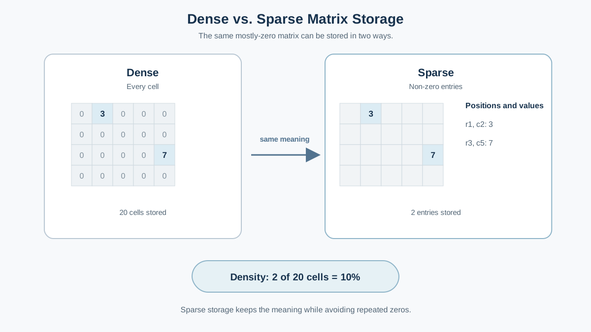
Here's where the mental model flips. Beginners often assume a mostly-zero matrix is wasteful. In the right format, it's the opposite: the zeros are what make it efficient.

A dense matrix stores every cell. If you have 100,000 rows and 300 one-hot encoded columns, that's 30 million values stored explicitly—even though roughly 29.7 million of them are zeros that all look identical.

A sparse matrix stores only what's non-zero. Instead of recording every cell, it records the position and value of each non-zero entry. For one-hot encoded data, that means storing one location per row instead of 300 values.

Think of it like a phone book. A dense representation is a grid with a cell for every possible phone number in existence—most of them empty. A sparse representation lists only the numbers that actually exist. Same information, radically different memory footprint.

This matters enormously at scale. A one-hot encoded matrix with thousands of categories might be impossible to hold in memory as a dense array. Stored sparsely, it becomes completely manageable. The same information fits in a fraction of the space because the zeros are implied rather than repeated.

Density is the measure that tells you how much you're saving. It's the fraction of entries that are non-zero. A 3-by-4 matrix with 12 cells and only 2 non-zero entries has a density of 2/12, or about 17%. The other 83% of its cells are zeros that a sparse format never needs to store.

Scikit-learn uses sparse matrix formats internally, and many of its estimators accept sparse input directly. When you see a warning or note about sparse matrices in the documentation, this is what it's referring to: a storage format that assumes most entries are zero and exploits that assumption.

Which Models Work Well with Sparse Data

Now we're at the third question: how does the estimator behave? This is where beginners need the most careful guidance, because the answer depends on the algorithm's math, not just its ability to accept a sparse format.

Regularized linear models are a strong default for high-dimensional sparse features. A model like Lasso does two useful things: it tends to drive many coefficients to zero, and it can compute efficiently on sparse input because it skips the zeros entirely. Regularization—a penalty that discourages overly large or numerous coefficients—helps control the complexity that comes with having far more features than rows.

Tree-based models split on individual features, one at a time. When most columns are rarely non-zero, a tree may not find enough clean split opportunities in a sparse but highly predictive column. This is not a universal rule—tree implementations differ, and some handle sparse input better than others. Treat it as a hypothesis to test, not a fact to memorize.

Distance-based models like k-nearest neighbors treat zeros as meaningful similarity. Two rows that share the same set of zeros look similar, which can be useful or misleading depending on your problem. If absence of a feature genuinely means "these items are alike," distance-based methods can work well. If absence is common across nearly everything, the distance signal washes out.

Here's the decision rule I'd give a beginner: start with a regularized linear baseline when your features are high-dimensional indicators or counts, then validate alternatives against it. Sparse compatibility is not proof of predictive suitability. The only reliable test is whether the model generalizes on your data.

Preprocessing Mistakes That Destroy Sparsity

The silent failure mode in sparse data work is densification: a preprocessing step that converts your efficient sparse matrix into a bloated dense one.

Scaling and imputation operations are common culprits. Some transformers expect dense input and will materialize the full matrix if you apply them carelessly. What worked fine on a small sample suddenly crashes or crawls on the full dataset—not because your data changed, but because your matrix format did.

The practical rule: keep the matrix sparse through encoding and transformation. Only densify deliberately, when the model or step genuinely requires it.

Here's the symptom to watch for: a pipeline that ran fine on a small sample grinds to a halt or throws a memory error on the full sparse dataset. That's not random bad luck. That's a hidden dense conversion.

Warning: Before you scale or transform a sparse matrix, check whether the operation preserves sparsity. If it forces a dense array, you may be multiplying your memory usage by hundreds or thousands.

This connects to feature scaling, but the order matters: scaling decisions affect your model, while matrix format affects whether your pipeline runs at all. Format first, scaling second.

When Sparse Data Is a Real Problem

Sparse data is not always benign. There's a genuine failure mode, and it's important to name it honestly.

The problem arises when non-zero values are so rare that most features carry almost no signal. With far more features than informative rows, a model can memorize the training data rather than learn general patterns. This is overfitting, and sparse, high-dimensional data is fertile ground for it.

The key distinction is between two kinds of sparsity:

• Structural sparsity comes from your encoding choices: one-hot categories, word counts, indicator flags. The zeros are meaningful, and the structure is informative.
• Signal sparsity means you genuinely lack enough non-zero observations to learn from. The features are mostly empty of predictive content, not just mostly zero.

Structural sparsity is usually fine—even beneficial—when you match it with the right model. Signal sparsity is a real problem that no storage format can fix.

How can you tell which one you have? Watch your validation performance. If your model scores well on training data but poorly on validation data, or if coefficients are unstable across runs, signal sparsity may be the culprit. That's when dimensionality reduction or feature selection becomes the right response—not because sparsity is inherently bad, but because your features lack real signal.

Working with Sparse Data in Practice

Here's a mental workflow you can carry into your next project:

Recognize when your pipeline produces sparse output. One-hot encoding and text vectorization both create sparse matrices. That's expected. Keep them sparse.

Know what your tools accept. Scikit-learn estimators generally accept sparse input. Some preprocessing steps preserve sparsity; others don't. When in doubt, check the documentation before you transform.

Inspect your matrix after each transformation. Check the object type, the shape, and the number of non-zero entries. If a step that should preserve sparsity suddenly produces a dense array, you've found the culprit.

Match your model to your data. For high-dimensional sparse features, regularized linear models are a strong baseline. Trees may need more thought. Distance-based methods depend on whether zeros carry similarity meaning.

Reduce dimensions only when signal sparsity is the real problem. If structural sparsity is working fine, dimensionality reduction can discard useful information without solving anything.

Tip: After you one-hot encode a categorical column, check the density of the resulting matrix. If it's below a few percent non-zero, you're working with sparse data—and you should treat it accordingly.

The Decision Rule That Matters

Here's the durable takeaway: treat zeros as information, keep the matrix sparse through encoding and transformation, match the algorithm to the sparsity, and only densify or reduce dimensions when signal sparsity—not structural sparsity—is the actual problem.

Your next step is concrete: inspect the density of your own one-hot encoded matrix. Trace where it stays sparse and where it silently densifies. That single habit will save you more debugging time than any model-tuning tip, because the failure mode you're avoiding is invisible until your pipeline crashes.

References

Research updated Sep 8, 2026