
Test Whether an Interaction Feature Helps a Model
Add a product term, watch the validation score tick up, declare victory. I have watched this exact sequence produce a confident conclusion on a dataset…

Key topics
Add a product term, watch the validation score tick up, declare victory. I have watched this exact sequence produce a confident conclusion on a dataset where no interaction existed. The score still went up. That is the trap: a single number cannot tell you whether you found signal or just got lucky.
So we are going to build a test that can tell those two situations apart. The plan is a controlled experiment. You generate data where you know whether an interaction exists, then check whether your workflow detects it when present and stays quiet when absent.
Why a Score Bump Is Not Proof
When a score improves after you add a feature, there are at least three explanations:
- Real signal. The feature captures a joint effect the model could not represent before.
- Noise fitting. The model latched onto random structure that will not repeat.
- Evaluation variance. You got a favorable split, and the same model would score differently on another sample.
A single train/test split cannot separate these. The only way to separate them is to control the data-generating process so you know the ground truth before you fit anything.
That gives us a clear success criterion. The interaction model should win on data with a real interaction and not reliably win on data without one. If your workflow passes both checks, it is measuring something real. If it fails either one, you are reading noise.
We compare two models: an additive baseline using only the main effects, and the same model plus an explicit product feature.
Prerequisites and Setup
You should already know what an interaction is and have run a leakage-safe validation workflow before. If the concept is fuzzy, the mental model is simple: an additive model cannot represent a joint effect, because it treats each feature's contribution as independent. That is exactly why we test instead of assume.
You need Python with NumPy, pandas, and scikit-learn. No external services, no credentials. Fix the random seed so every number here reproduces on your machine.
import numpy as np
import pandas as pd
from sklearn.linear_model import LinearRegression
from sklearn.model_selection import train_test_split, cross_val_score
from sklearn.pipeline import Pipeline
from sklearn.preprocessing import FunctionTransformer

RANDOM_STATE = 42
Build a Dataset With a Known Interaction
We define the target as a sum of main effects plus a product term. The coefficient on the product is the knob that controls interaction strength.
def make_data(n=500, interaction_coef=2.0, noise=1.0, seed=42):
    rng = np.random.default_rng(seed)
    x1 = rng.normal(0, 1, n)
    x2 = rng.normal(0, 1, n)
    y = 1.5 * x1 + 0.8 * x2 + interaction_coef * (x1 * x2) + rng.normal(0, noise, n)
    return pd.DataFrame({"x1": x1, "x2": x2, "y": y})

df = make_data(interaction_coef=2.0)
print(df.head())
You get a small frame with x1, x2, and a target whose values depend on both features jointly. When interaction_coef is zero, the target is purely additive.
Knowledge check
Check your understanding
Answer this question before you continue.
Fit the Additive Baseline
Split before any fitting, then train a linear model on x1 and x2 only. By construction, this model family cannot represent the product term.
X = df[["x1", "x2"]]
y = df["y"]

X_train, X_test, y_train, y_test = train_test_split(
    X, y, test_size=0.2, random_state=RANDOM_STATE
)

baseline = LinearRegression().fit(X_train, y_train)
print("baseline R2:", baseline.score(X_test, y_test))
The baseline is misspecified for this target. It is not a bad model; it is the wrong shape for a target that bends with the product of two features. Expect a score clearly below the interaction model.
Add the Interaction Feature
The product feature is a fixed row-wise calculation: x1 * x2 for each row, with no statistics learned from the data. Computing it before the split does not leak anything, because no row's value depends on any other row. That distinction matters, and it is worth stating plainly because the leakage rule gets applied too broadly.
Where the pipeline earns its keep is workflow integrity. It bundles the representation with the estimator so the two travel together, and it protects you the moment you add a preprocessing step that does learn from data, such as scaling or target encoding. Keep the transform inside the pipeline as a habit, not because this particular product needs it.
def add_product(X):
    X = np.asarray(X)
    return np.hstack([X, (X[:, 0] * X[:, 1]).reshape(-1, 1)])

interaction_model = Pipeline([
    ("product", FunctionTransformer(add_product)),
    ("model", LinearRegression()),
])

scores = cross_val_score(interaction_model, X_train, y_train, cv=5, scoring="r2")
print("interaction CV R2:", scores.mean(), "+/-", scores.std())
Common mistake: Assuming every transformation outside a pipeline leaks. A stateless row-wise product does not. A transformation that estimates parameters from the training data — a scaler's mean, a target encoder's category statistics — does, and that is the case the pipeline rule exists to prevent.
Knowledge check
Check your understanding
Answer this question before you continue.
Compare Both Models on the Same Folds
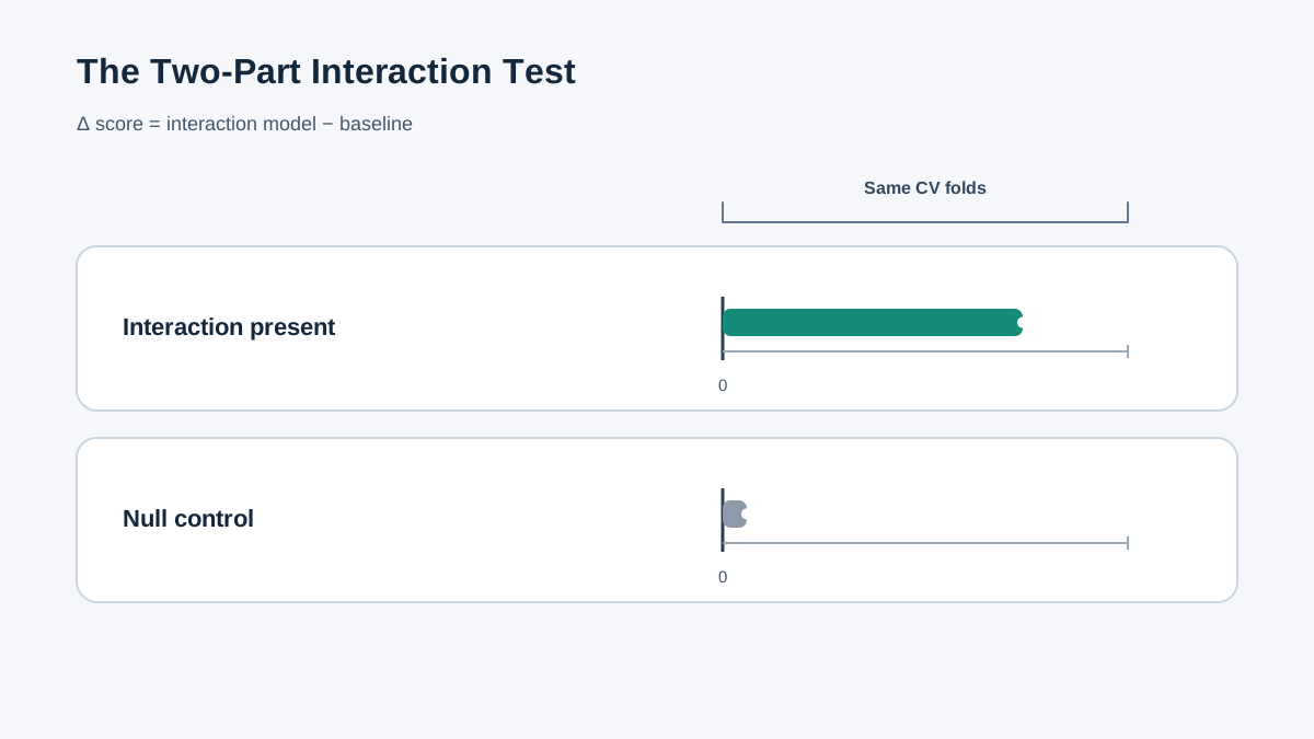
The baseline above was scored on a held-out test set, while the interaction model was scored by cross-validation on the training set. Those are different samples and different procedures, so the gap between them is not a clean estimate of the feature's benefit. Fix that before drawing any conclusion.
Score both models with the same cross-validation call on the same data:
base_cv = cross_val_score(baseline, X_train, y_train, cv=5, scoring="r2")
inter_cv = cross_val_score(interaction_model, X_train, y_train, cv=5, scoring="r2")

print("baseline CV R2:   ", base_cv.mean(), "+/-", base_cv.std())
print("interaction CV R2:", inter_cv.mean(), "+/-", inter_cv.std())
print("gap:", inter_cv.mean() - base_cv.mean())
Now the two numbers come from the same folds, the same scoring function, and the same rows. The gap is comparable. You want it to be larger than the fold-to-fold variation in either model, not merely positive.
Knowledge check
Check your understanding
Answer this question before you continue.
Run the Same Test on Data With No Interaction
This is the control. Regenerate the data with interaction_coef=0.0 and keep everything else identical, including the evaluation procedure.
df_null = make_data(interaction_coef=0.0)
X_null = df_null[["x1", "x2"]]
y_null = df_null["y"]

X_tr, X_te, y_tr, y_te = train_test_split(
    X_null, y_null, test_size=0.2, random_state=RANDOM_STATE
)

base_null = LinearRegression().fit(X_tr, y_tr)
base_null_cv = cross_val_score(base_null, X_tr, y_tr, cv=5, scoring="r2")
inter_null_cv = cross_val_score(interaction_model, X_tr, y_tr, cv=5, scoring="r2")

print("baseline CV R2:   ", base_null_cv.mean(), "+/-", base_null_cv.std())
print("interaction CV R2:", inter_null_cv.mean(), "+/-", inter_null_cv.std())
print("gap:", inter_null_cv.mean() - base_null_cv.mean())
Here the two models should perform about the same, and any difference should sit inside the noise band. This is a check, not proof. One run on one seed is a single sample of a noisy process. To treat it as evidence, repeat the whole experiment across several seeds and confirm the null gap stays near zero while the real-interaction gap stays positive.
Knowledge check
Check your understanding
Answer this question before you continue.
Read the Result Without Overclaiming
A win on one controlled dataset is evidence about that data-generating process, not a universal rule about interaction features. Keep three distinctions in mind:
- Statistical vs practical significance. A small but consistent gain may not justify the added complexity or the loss of interpretability.
- Scope. Results depend on sample size, noise level, model family, and how the interaction is encoded.
- Mechanism. A linear model needs the explicit product. A tree-based model can often capture the same interaction without one.
My decision rule: only add an explicit interaction when the gain survives both the control dataset and a stability check across folds and seeds.
Failure Modes and Debugging Signals
| Symptom | Likely cause |
|---|---|
| Score gap vanishes when you change the seed | The effect was noise |
| Interaction model wins on both datasets | Leakage or an evaluation bug |
| Both models score near chance | Check target construction and feature scaling |
| Folds disagree wildly | Dataset too small or too noisy for a stable conclusion |
When a gap disappears under a new seed, that is not a failure of your experiment. It is the experiment doing its job.
One Modification to Try Next
Sweep the interaction coefficient from zero upward and plot the score gap against interaction strength. Use the same cross-validation procedure for both models at every value.
for coef in [0.0, 0.5, 1.0, 2.0, 4.0]:
    d = make_data(interaction_coef=coef)
    Xd, yd = d[["x1", "x2"]], d["y"]
    Xtr, Xte, ytr, yte = train_test_split(Xd, yd, test_size=0.2, random_state=RANDOM_STATE)
    base = cross_val_score(LinearRegression(), Xtr, ytr, cv=5, scoring="r2").mean()
    inter = cross_val_score(interaction_model, Xtr, ytr, cv=5, scoring="r2").mean()
    print(f"coef={coef}: baseline={base:.3f} interaction={inter:.3f} gap={inter-base:.3f}")
You will see a threshold where the interaction model starts to reliably win. That turns a single yes/no result into a curve showing how detectability depends on effect size and noise. As an extension, swap the linear model for a tree-based model and note that it can capture the interaction without an explicit product feature.
The reusable rule is this: never trust one score change. Run the controlled test, check the no-interaction control, verify stability across folds and seeds, and only then decide whether the added representation earns its place. Your next step is to run this same workflow inside a real pipeline on your own data, where you do not know the ground truth and the control dataset has to be your discipline instead.
Knowledge check
Final check
Finish the article by checking the ideas you just learned.
References
Build stronger machine learning foundations
Use structured resources to connect theory, scikit-learn workflows, and evaluation practice.


