
Feature-Hashing Collisions: Probability, Buckets, and Memory Tradeoffs
You picked 2^18 buckets. You trained the model. The metrics came back slightly worse than your explicit-vocabulary baseline, and now you are staring at the…

Key topics
You picked 2^18 buckets. You trained the model. The metrics came back slightly worse than your explicit-vocabulary baseline, and now you are staring at the gap wondering whether it is collision damage, ordinary noise, or a hyperparameter you set badly.
The problem is not the gap. The problem is that you have no model for what the gap should be. So let's build one. By the end of this article you will be able to compute the probability that your token set contains a collision, estimate how many colliding pairs to expect, and read those numbers as a memory decision instead of a defect report.
The Question Behind the Question
The literal question is "how many collisions will I get?" The hidden question is "how many buckets do I need before collisions stop mattering?"
If you already understand the hashing trick mechanically — each token maps to one of B columns with no stored vocabulary — then you know the representation width is fixed at B no matter how many distinct tokens appear. That fixed width is the entire point. It is also the source of the tax.
Three quantities govern everything that follows:
- B — the number of buckets, meaning the number of columns in the hashed representation.
- n — the number of distinct tokens you actually hash.
- p — the probability that at least one pair of distinct tokens lands in the same bucket.
One assumption carries the whole derivation: treat the hash function as producing uniform, independent bucket assignments. Real hash functions approximate this. A badly chosen hash or an adversarially seeded one can violate it, and when that happens the math below stops describing your system.
Two boundaries before we start. This article derives collision probability and memory cost. It does not claim collisions are always harmful, and it does not claim they are reversible — the hasher keeps no inverse mapping, so once two tokens share a column, you cannot pull them apart.
Notation and the Bounded Hashing Model
Under the uniform-independent assumption, the probability that any specific pair of distinct tokens collides is exactly 1/B. That number is almost never the one you care about.
What you care about is the probability that some pair collides, anywhere in your token set. Those are different questions. The first is a coin flip on one pair. The second is a statement about the whole system, and it grows much faster than intuition suggests.
Here is the pigeonhole framing: with n tokens and B buckets, once n approaches the scale of B, collisions are not an edge case. They are the expected state of the system. You would need B to be astronomically larger than n to make collisions genuinely rare.
The second mental handle is occupancy. Instead of counting colliding pairs, count how many buckets stay empty and how many hold more than one token. Both views describe the same system. The pair view is easier to derive from. The occupancy view is easier to picture when you are deciding whether your bucket count is sane.
Note: The assumption that breaks first in practice is uniformity of tokens. Natural language has a heavy head and a long tail. The derived probability depends on how many distinct tokens you assign, not on how often they occur. Token frequency changes how consequential a collision is, not how likely it is. A rare token colliding with another rare token barely moves the model; a frequent, high-signal token colliding with another frequent token forces two well-determined coefficients into one blended weight.
Knowledge check
Check your understanding
Answer this question before you continue.
Deriving the Collision Probability
Start from the complement. Compute the probability that all n tokens land in distinct buckets, then subtract from 1.
The first token is always free. It cannot collide with anything because nothing is there yet. The second token avoids one occupied bucket out of B, so it lands distinct with probability (B−1)/B. The third avoids two occupied buckets: (B−2)/B. And so on.
Each factor is a conditional probability given that the earlier tokens already occupied distinct buckets. The factors are not independent — the available bucket count shrinks with each token — but the chain rule of conditional probability lets us multiply them to get the joint probability that all n tokens are distinct:
So the collision probability is:
That product is exact, and it is also a numerical trap. For large n it underflows, and computing it directly in floating point loses precision long before you reach realistic vocabulary sizes. The practical form is the exponential approximation:
The n(n−1)/2 structure comes straight out of the product: it is the number of distinct pairs among n tokens. That is where the birthday problem lives.
Now the rule of thumb that falls out of the math, and the single most useful number in this article: collisions become likely on the order of the square root of B tokens, not on the order of B tokens.
If you have a million buckets, you should expect meaningful collision pressure somewhere around a thousand distinct tokens — not a million. That is the cliff, and it arrives far earlier than most people guess.
Connect the symbol back to the mechanism. When p is the probability that at least one pair shares a column, the consequence is that their contributions to that column are summed. The model can no longer separate them. That is what a collision is.
Knowledge check
Check your understanding
Answer this question before you continue.
A Worked Example You Can Check by Hand
Pick something tiny so you can verify the formula yourself. Let B = 100 and n = 10.
The exact product gives:
So p ≈ 0.372, roughly a 37 percent chance that at least one pair collides.
The approximation gives:
Close enough. The approximation is trustworthy in the regime that matters, and it does not blow up when you scale it.
Now scale it. Suppose you have 50,000 distinct tokens — a reasonable text-classification vocabulary — and you are choosing between bucket counts that are powers of two.
| Buckets (B) | √B | p at n = 50,000 |
|---|---|---|
| 2^16 = 65,536 | ~256 | effectively 1.0 |
| 2^18 = 262,144 | ~512 | effectively 1.0 |
| 2^20 = 1,048,576 | ~1,024 | effectively 1.0 |
| 2^22 = 4,194,304 | ~2,048 | ~1.0 |
| 2^24 = 16,777,216 | ~4,096 | ~1.0 |
Every one of these is essentially certain to contain at least one collision. That is not a failure of the table. It is the point: the probability that at least one pair collides is the wrong number to optimize once n is large. At 50,000 tokens, you will have collisions no matter what. The question becomes how many, and how much signal they mix.
That reframes the whole exercise. The birthday-problem probability tells you when collisions start. It does not tell you when they start to matter. For that, you need the expected number of colliding token pairs, which is approximately n(n−1)/(2B).
At n = 50,000 and B = 2^20, that is about 1,192 colliding pairs. At B = 2^18, it is about 4,768. Four times as many, because halving B doubles the expected pair count.
Common mistake: Reading a collision probability near 1.0 and concluding the representation is broken. A near-certain existence of at least one collision is normal and expected. What matters is the expected pair count and whether the collisions land on tokens whose signal you actually need.
The honest limit: this computation assumes uniform hashing and treats all tokens as equally important. It gives you an order-of-magnitude decision, not a precise prediction of your model's accuracy.
Knowledge check
Check your understanding
Answer this question before you continue.
From Collision Probability to Memory
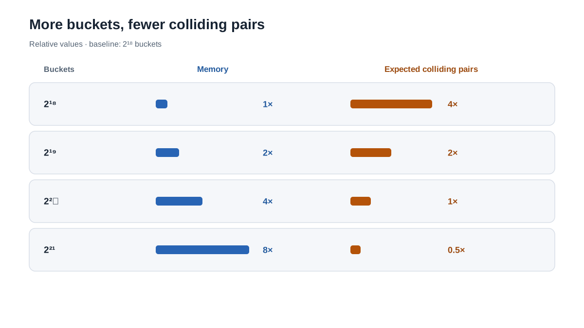
Here is the memory model, stated plainly: the representation cost scales with B, not with the vocabulary size. That is the entire reason feature hashing exists. You trade a growing index for a fixed width.
Two components deserve separate attention.
The index and value arrays of the sparse matrix scale with the number of non-zero entries per row — how many tokens are actually present in a given document. That number does not change when you change B.
The column dimension B sets the width of the matrix and, for a linear model, the number of learned parameters. That number scales linearly with B.
So doubling B roughly halves the expected colliding-pair count, but it doubles the column dimension and therefore the model's parameter count. The marginal return on extra buckets shrinks as B grows, because you are paying linearly for a benefit that decays.
| B | Relative memory | Relative expected colliding pairs |
|---|---|---|
| 2^18 | 1× | 4× |
| 2^19 | 2× | 2× |
| 2^20 | 4× | 1× |
| 2^21 | 8× | 0.5× |
The practical reading: choose B so the expected colliding-pair count sits in a range you can tolerate, then stop paying for buckets. Past that point you are buying memory, not accuracy.
This is the sparse representation memory tradeoff in its cleanest form. A wider B with the same non-zero count keeps the matrix sparse, so the cost shows up mostly in model parameters and index width rather than in stored values.
Knowledge check
Check your understanding
Answer this question before you continue.
What Collisions Actually Do to the Model
A collision sums the contributions of two tokens into one column. For a linear model, that means the learned weight is a compromise between two tokens' effects. The model can still learn. It just learns a blended coefficient.
Why is that often tolerable? Because rare tokens collide with other rare tokens, and their individual weights were weakly determined anyway. The damage concentrates when a frequent, high-signal token collides with another frequent token — that is where two well-determined coefficients get forced into one.
The real failure mode is subtler than "noise." Collisions are not random noise you can average away, because the same pair collides on every row. The error is systematic and consistent. That is why it can quietly cap accuracy rather than merely add variance. Your validation curve looks fine; your ceiling is just lower than it should be.
And the irreversibility is absolute. The hasher has no inverse mapping. You cannot recover which token contributed what. If you need per-token interpretation or per-token weights, feature hashing is the wrong tool.
When not to use this: Skip feature hashing when individual token attribution is a requirement, or when your vocabulary comfortably fits in an explicit index. The tradeoff only pays off when the vocabulary is large, unstable, or streaming — and when you can accept blended coefficients.
Choosing a Bucket Count in Practice
Here is the procedure I would run on my own data.
Step one: Estimate n from a sample, not from a guess. Count distinct tokens in a representative slice of your corpus.
Step two: Pick a candidate B and compute the expected colliding-pair count with n(n−1)/(2B). That number tells you the scale of collisions to expect. The per-pair collision probability under the model is simply 1/B — useful as a baseline, but it does not tell you how many collisions your full token set will contain.
Step three: Sanity-check against the square-root rule. If n is anywhere near √B, expect meaningful collisions and consider widening.
Step four: Verify empirically. Compare a hashed representation against an explicit-vocabulary baseline on a held-out split, and treat the gap as the measured cost of the memory you saved. This is where token frequency enters the picture: a frequency-aware comparison shows whether the collisions are landing on tokens that carry signal.
Step five: Remember that collision probability is a property of the representation, not of the model. Changing the classifier will not change which tokens share a column.
The Better Question
You came in asking how to avoid collisions. The better question is how much collision probability you are willing to buy with memory.
Two numbers carry that decision. The square-root threshold tells you when collisions start. The linear scaling of memory with B tells you what each additional bucket costs. Everything between those two facts is arithmetic you can do before you train anything.
So do it. Estimate the distinct token count on a sample of your own data. Compute the expected colliding-pair count for two candidate bucket counts. Compare both against an explicit-vocabulary baseline on a held-out split, and inspect whether the collisions are landing on frequent tokens or on the long tail. Then pick the bucket count whose measured cost you are willing to pay.
Collisions are a priced tradeoff, not a defect. The price is computable, and you can read it off the back of an envelope before the first model ever fits.
Knowledge check
Final check
Finish the article by checking the ideas you just learned.
References
Build stronger machine learning foundations
Use structured resources to connect theory, scikit-learn workflows, and evaluation practice.


