The Curse of Dimensionality: Why More Features Can Make Distance Useless

You add more columns to your dataset expecting a better model. Instead, your k-nearest neighbors accuracy drops, your clusters turn to mush, and every point suddenly looks equally close to every other point. This is the curse of dimensionality—and it is not a warning about having too much information. It is a warning about what happens to geometry when you add dimensions faster than you add data.

The weak mental model goes like this: more features mean more information, and more information means a better model. The reality is more subtle. Features add volume to your feature space faster than they add signal, and distance-based methods pay the price first. The real question is not "how many features should I have?" but "what is my actual constraint—sparsity, distance collapse, or overfitting?"

The Symptom: More Features, Worse Neighbors

Here is the recurring beginner experience. You have a dataset with a few columns, and your KNN model performs reasonably. You add a handful of new features—maybe some interaction terms, a few aggregated statistics, a couple of encoded categories—and retrain. Accuracy drops. Clustering quality degrades. The model that should have more information to work with somehow got worse.

This feels like a betrayal of intuition. It is not. The problem is that KNN and other distance-based methods do not learn a global rule from your data. They make predictions by finding nearby points and asking what those neighbors say. "Nearby" is a geometric claim, and geometry behaves strangely when the space gets wide.

The reframe is simple: each feature you add multiplies the volume of the space your data lives in, but your number of samples stays fixed. Your points spread out like a handful of marbles dropped into an expanding warehouse. Distance-based methods run short of trustworthy neighbors because the neighbors are no longer actually near.

Volume Grows Faster Than Data: The Sparsity Problem

Start with the simplest version of the problem. Ten points can cover a line with reasonable density. To keep that same density in a square, you need about 100 points. In a cube, about 1,000. In ten dimensions, you need 10 billion.

That is the curse of dimensionality explained in its most concrete form: the volume of a high-dimensional space grows exponentially with each new dimension, so a fixed number of points becomes exponentially sparse.

Sparsity matters because distance-based methods depend on density. KNN works by finding the closest examples to a query point and letting them vote. Clustering works by grouping points that are close together. Density-based methods like DBSCAN connect points within a fixed neighborhood radius. All of these approaches assume that nearby points exist and that they carry useful information. In a sparse space, "nearby" becomes a rare commodity.

A useful way to picture this: imagine trying to find your friends in a stadium. In a small stadium with a few hundred people, you can scan the crowd and spot familiar faces. In a stadium the size of a city, with the same few hundred people scattered across the seats, you could walk for hours and never find anyone you know. The people did not disappear. The space just got too large for the number of people in it.

The boundary of this analogy matters. Sparsity is not about the raw feature count alone. It is about the ratio of samples to volume. A dataset with 100,000 rows and 50 features may be perfectly dense for your purposes, while a dataset with 1,000 rows and 10 features may already be too sparse. The curse bites when your sample size cannot keep pace with the space your features create.

Distance Concentration: When Every Point Is Equally Far

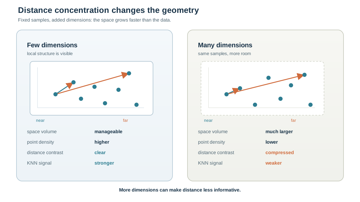
Sparsity is intuitive. Distance concentration is not, and it is the more damaging of the two effects.

Here is the phenomenon: as dimensions grow, the pairwise distances between points converge. The nearest neighbor and the farthest neighbor become nearly the same distance away. If every point is equally far from every other point, then "nearest" loses its meaning.

This is not a data-volume problem. You can add more samples and slow the effect, but you cannot eliminate it. Distance concentration is a property of how distances behave in high-dimensional geometry. When features are independent and noisy, the distance between any two points is dominated by the accumulation of small differences across many dimensions. The signal that one point is genuinely closer than another gets buried under the noise of all the dimensions where the points differ slightly.

Think about it operationally. In two dimensions, you can look at a scatter plot and see which points cluster together. In three dimensions, you can rotate a plot and still see structure. In fifty dimensions, you cannot visualize the space at all, and the math is working against you: the ratio of the distance to the nearest neighbor over the distance to the farthest neighbor approaches 1 as dimension increases. When that ratio hits 1, every point is effectively equidistant, and proximity ranking becomes a coin flip.

Research adds an important nuance here. Distance concentration is most severe when features are independent and noisy. When features are correlated or genuinely informative, distances can retain contrast. This is why the curse is not an absolute wall—it is a warning about what happens when you pile on dimensions without considering whether they carry signal or just volume.

Why Some Models Survive High Dimensions

The curse is not universal. It hits methods whose predictions depend directly on pairwise distance, neighborhood, density, or similarity calculations. KNN, k-means clustering, and DBSCAN all degrade first when distances lose contrast. Kernel methods can suffer too, but their behavior depends heavily on the kernel and the representation—some kernels effectively reshape the space in ways that resist the effect.

Linear models and regularized models are far more tolerant. A linear model does not ask "who is near this point?" It learns a set of weights that map features to predictions. Adding many features increases the risk of overfitting, but regularization can control that risk by penalizing large weights. The model does not depend on local geometry, so distance concentration does not directly break it.

Tree ensembles sit somewhere in between. They are relatively robust to irrelevant features because each split considers one feature at a time, and the model can ignore unhelpful dimensions. They still face overfitting risk in high dimensions, but they do not suffer the same collapse as distance-based methods.

The decision rule that falls out of this: match the model family to the constraint. If your data is high-dimensional and your method is distance-based, you are fighting the geometry itself. If your method is linear or tree-based, your problem is more likely variance and overfitting—a different disease with a different treatment.

Choosing a Response: Reduce, Regularize, or Switch

When a distance-based model degrades as features grow, diagnose the constraint first, then pick the response that targets it.

Feature selection is the cheapest and most interpretable option. If you can identify irrelevant or redundant features, drop them. This works best when you have domain knowledge or when simple filters reveal that some columns carry no signal. Feature selection does not change your features—it removes the ones that are not earning their keep.

Dimensionality reduction compresses correlated variation into fewer dimensions. Principal component analysis finds directions of maximum variance and projects your data onto them. This can help when you have many features that are largely redundant, but treat it as a hypothesis to test, not a guaranteed repair. PCA preserves directions of variance, not necessarily class separation or neighborhood structure. High-variance directions can be nuisance variation. The mechanics of PCA deserve their own treatment—the key point here is that reduction is a response to the curse, not a cure for every modeling problem.

Regularization is the answer when you want to keep many features but control variance. Ridge and lasso regression penalize model complexity, shrinking weights and forcing the model to rely on the features that actually predict. This works for linear models and some others, but it does not rescue distance-based methods, because regularization does not fix the geometry.

Switching model families is sometimes the honest answer. If your data is genuinely high-dimensional and your task is classification, a regularized linear model or a tree ensemble may simply be a better fit than KNN. The local-versus-global tradeoff matters here: distance-based methods excel when local structure is informative, but they fail when the space is too wide for locality to mean anything.

Warning: Do not apply PCA or feature selection blindly. Check whether your model actually suffers from high dimensions first. If a regularized linear model handles your 500-feature dataset fine, you do not have a dimensionality problem—you have a different model family that already tolerates the space.

Common Mistakes and How to Spot Them

Mistake 1: Assuming more features always help. The symptom is validation performance dropping as you add columns. Watch your cross-validation scores as you expand your feature set. If accuracy rises then falls, you are watching the curse arrive.

Mistake 2: Blaming the model when the real issue is feature quality. A bad KNN result in high dimensions might be a geometry problem, or it might be that half your features are noise. Check feature quality before you abandon the approach. If you drop the noisy columns and performance recovers, the problem was signal, not space.

Mistake 3: Applying dimensionality reduction without scaling features first. PCA and most distance-based methods assume features are on comparable scales. If one feature ranges from 0 to 1 and another from 0 to 1,000, the second dominates every distance calculation. Standardize your features before reduction or distance computation.

Mistake 4: Treating the curse as a reason to avoid features entirely. Sometimes the signal genuinely lives across many dimensions. Text data, image data, and many sensor datasets are high-dimensional by nature, and the information is distributed across the full feature space. The curse is a warning about the ratio of samples to volume, not a prohibition on having many columns.

When the Mental Model Breaks Down

The curse of dimensionality is not a hard threshold. It depends on the ratio of samples to intrinsic dimension—the number of dimensions your data actually varies along—not the raw feature count. A dataset with 1,000 features that are all highly correlated may behave like a dataset with 5 effective dimensions. A dataset with 20 independent features and few samples may suffer terribly.

Correlated and informative features behave differently than independent noisy ones. When features carry real signal, distances can retain contrast even in high dimensions. The research is clear on this point: the curse is most severe when dimensions are independent and noisy, and feature selection can restore meaningful distance contrast.

Some modern methods operate comfortably in very high dimensions. Deep learning models routinely handle inputs with thousands or millions of dimensions because they learn hierarchical representations that compress the relevant structure. The curse is not a universal wall—it is a specific failure mode of distance-based classical methods when the space outgrows the data.

The mental model predicts where classical distance-based methods struggle. It does not predict where all learning fails.

The Decision Rule

When a distance-based model degrades as features grow, run this diagnosis:

1. Is the space sparse? Compare your sample count to your feature count. If you have far more dimensions than samples, sparsity is likely biting.
2. Are distances collapsing? Check the ratio of nearest-neighbor distance to farthest-neighbor distance. If it is near 1, distance concentration has destroyed the signal.
3. Is the model overfitting? If training performance is high but validation performance is low, you have a variance problem, not a geometry problem.

Then respond accordingly: feature selection when you can identify the useless columns, dimensionality reduction when features are redundant, regularization when you want to keep the features but control variance, and a different model family when the geometry itself is the constraint.

The fastest way to internalize this is to run a small experiment. Generate a dataset with a few informative features, then add random noise columns one at a time. Watch your KNN accuracy decline as the noise dimensions accumulate. Then run PCA and watch the contrast return. The curse of dimensionality stops being abstract the moment you watch it happen in your own output.

References

Research updated Sep 8, 2026