
Feature Interactions in Machine Learning: When Variables Work Together
You fit a linear model. The coefficients look sensible. Each feature seems to contribute its own share, and the numbers align with your intuition. Then you…

Key topics
You fit a linear model. The coefficients look sensible. Each feature seems to contribute its own share, and the numbers align with your intuition. Then you check the validation score, and the model is still missing something. Not because the data is noisy, but because the pattern you are trying to predict only appears when two features are considered together.
This is the classic signature of a feature interaction, and it is one of the most common reasons a perfectly reasonable linear model quietly underperforms.
The symptom: a model that misses what each variable alone cannot explain
Imagine you are predicting house prices. You have two features: square footage and neighborhood quality. You fit a linear regression, and the coefficients look healthy. Bigger houses cost more. Better neighborhoods cost more. The model is not broken, yet it keeps underpredicting the most expensive homes.
Here is what is happening: in the real market, location matters more for large houses than for small ones. A big house in a great neighborhood commands a serious premium. A big house in a mediocre neighborhood is just a big house. The effect of square footage depends on the value of neighborhood quality, and no single coefficient can capture that.
If you inspect individual feature importance, everything looks fine. Square footage is important. Neighborhood quality is important. But the model cannot see the joint effect because its prediction equation is additive: it adds each feature's contribution together as if they acted independently.
The diagnostic handle is simple: the effect of one feature changes depending on the value of another feature. When that is true, you have an interaction, and your additive model will miss it no matter how carefully you tune the coefficients.
Knowledge check
Check your understanding
Answer this question before you continue.
What an interaction actually is
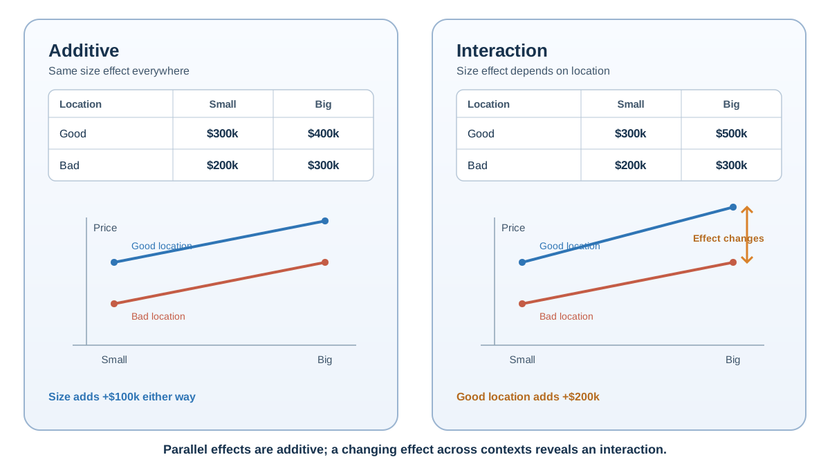
An interaction is the change in prediction that appears only after accounting for each feature's individual effect. It is the extra signal that emerges when two variables are considered together.
Let's make this concrete with a small example. Suppose you are predicting house value with two binary features: size (big or small) and location (good or bad). Here is an additive relationship, where each feature contributes a fixed amount:
| Location | Size | Predicted value |
|---|---|---|
| Good | Big | $350,000 |
| Good | Small | $200,000 |
| Bad | Big | $250,000 |
| Bad | Small | $100,000 |
Read the rows carefully. Moving from small to big adds $150,000, regardless of location. Moving from bad to good adds $100,000, regardless of size. The effects are constant. That is additivity: each feature contributes its own fixed share, and the total is simply the sum.
Now consider an interacting relationship:
| Location | Size | Predicted value |
|---|---|---|
| Good | Big | $450,000 |
| Good | Small | $200,000 |
| Bad | Big | $250,000 |
| Bad | Small | $100,000 |
In a bad location, going from small to big adds $150,000. In a good location, it adds $250,000. The size effect changed because the location changed. That extra $100,000 on top of the expected additive total is the interaction.
A useful way to visualize this is with two lines. Plot size on the x-axis and predicted value on the y-axis, with one line for good locations and one for bad. In an additive model, the lines are parallel. In an interacting model, they cross or fan out. Parallel lines mean each feature contributes its own fixed share. Crossing or fanning lines mean the features are working together.
One clarification matters here: an interaction is a property of the true relationship you are trying to model, not of the data alone. Two features can be correlated without interacting. Correlation describes the relationship between features. Interaction describes how features jointly affect the target. These are separate ideas, and confusing them causes real problems.
Why additive models miss interactions
A linear model predicts with a weighted sum:
prediction = w1 * feature1 + w2 * feature2 + bias
Each feature contributes independently. Change feature1 by one unit, and the prediction changes by w1, regardless of what feature2 is doing. This additive structure cannot represent a joint effect, no matter how the coefficients are tuned. The limitation is representational, not a tuning problem.
If you have worked with polynomial regression, you might wonder whether adding squared terms helps. It does not, at least not for this problem. Adding a squared term like feature1² creates curvature in one feature, but it still cannot capture a product like feature1 * feature2. Polynomial terms bend a single feature's contribution. Interactions require combining different features.
Think of it this way: an additive model is a team where each member contributes their own fixed amount. An interaction is a team where the members amplify each other. No amount of adjusting individual salaries captures the synergy.
Knowledge check
Check your understanding
Answer this question before you continue.
How representation exposes interactions
You have two main routes to capturing interactions: engineer them into the features, or choose a model that learns them natively.
Route one: explicit interaction terms
Create a new feature that is the product of two existing features. For numeric features, multiply them: size * location_score. For categorical features, create a feature cross: combine every pair of category values into a new categorical value.
This is the categorical counterpart of polynomial terms. Where polynomial expansion adds powers of a single numeric feature, feature crosses combine two or more categorical or bucketed features. A linear model can then see the joint signal because the interaction has been made explicit.
The advantage is interpretability. Your model now has a coefficient for the interaction term, and you can read what the joint effect is worth. The disadvantage is that you have to guess which interactions matter. Domain knowledge helps here. If you have a reason to believe two features act together, an explicit term is a direct test of that belief.
Knowledge check
Check your understanding
Answer this question before you continue.
Route two: interaction-native models
Decision trees and tree ensembles can represent conditional effects through sequential splits. A tree might first split on neighborhood quality, then split on size differently within each branch. One branch learns "big house in good neighborhood" carries a premium, while another branch learns "big house in bad neighborhood" does not. The model discovers the interaction structure automatically, without you naming it in advance.
The tradeoff is interpretability. Tree ensembles find interactions you did not anticipate, which is powerful, but reading the learned structure back out of a forest of hundreds of trees is far harder than reading a single coefficient.
Here is my rule of thumb:
- Use explicit interaction terms when you have domain knowledge about which combinations matter, and when you need to explain the model to someone else.
- Use tree-based models when you suspect interactions exist but do not know where, and when predictive performance matters more than interpretability.
One boundary worth naming: the feature construction itself depends on your inputs. Numeric interactions are products. Categorical interactions are crosses of category values. And if you suspect the interaction only matters past a threshold, a tree model may capture that conditional structure more naturally than a hand-built product term.
Knowledge check
Check your understanding
Answer this question before you continue.
The trap: correlation is not interaction
Beginners often collapse three separate ideas into one: correlated features, nonlinear single-feature effects, and true interactions. They are different, and treating them as the same leads to wasted effort.
Correlated features can make your coefficients unstable. If two features move together, the model cannot cleanly attribute credit between them. This is a real problem, but it is not an interaction. Correlated features do not imply that the target depends on their combination.
A nonlinear single-feature effect, like a curved relationship between one feature and the target, is also not an interaction. Polynomial terms handle that. Interactions are about joint effects across different features.
The practical test for an interaction is always the same: does the effect of one feature change when the other feature changes? If the answer is no, you do not have an interaction, no matter how correlated the features are or how curved each individual relationship looks.
There is also a cost to adding interactions blindly. Each interaction term adds a parameter, which adds variance. If you throw in every pairwise product, you will fit the training data better and generalize worse. An interaction that only helps on training data is noise, not signal.
Common mistake: Treating a strong single-feature signal as evidence of an interaction. A feature can be highly predictive on its own and still have zero interaction with anything else.
A practical workflow for deciding whether to add interactions
Here is a repeatable path I use when a linear model underfits:
Start with domain reasoning. Ask which feature combinations plausibly act together in the real process. In housing, size and location. In credit risk, income and debt load. In healthcare, age and pre-existing conditions. Your knowledge of the problem is the cheapest source of interaction hypotheses.
Then let a flexible model act as a probe. Fit a tree ensemble alongside your linear baseline. If the tree model clearly beats the linear model on held-out data, the additive linear form is insufficient. That gap tells you something is missing, but it does not automatically prove interactions are the cause. The tree could be exploiting thresholds, piecewise behavior, or nonlinear single-feature relationships instead. Treat a large gap as a signal to investigate, not as proof of interaction structure.
If you need interpretability, add explicit interaction terms. Take your best domain-driven guesses, create the product features, and compare validation performance against the plain linear baseline. Let the held-out data decide whether each interaction earns its place.
Always validate on held-out data. Training performance will improve as you add terms. That is guaranteed. The question is whether the improvement survives on data the model has not seen. If it does not, the interaction was noise.
The decision rule is straightforward: let the model family match the structure you expect, and let validation, not intuition alone, decide whether an interaction earns its place.
When your linear model underfits, ask the question before reaching for more features or a bigger model: does the target depend on combinations of features, or on each feature separately? If combinations matter, choose between explicit interaction terms and a tree-based model based on whether interpretability or automatic discovery matters more. Then confirm the choice on held-out data.
The whole is greater than the sum of its parts, but only when the parts actually work together. Your job is to find out whether they do.
Knowledge check
Final check
Finish the article by checking the ideas you just learned.
References
Research updated Sep 8, 2026


