Ridge Regression: Derive the Penalized Least-Squares Solution

Two features that measure almost the same thing can make ordinary least squares produce coefficients that swing wildly while the predictions barely move. Ridge regression fixes that by adding one term to the objective. Here is the derivation, step by step.

Why OLS Breaks Down When Features Collide

You already know the ordinary least-squares solution. Minimize the residual sum of squares, set the gradient to zero, and you land on the normal equations:

$X^\top X \hat{\beta} = X^\top y \quad\Longrightarrow\quad \hat{\beta}_{\text{OLS}} = (X^\top X)^{-1} X^\top y$

That inverse is the whole story. Everything depends on $X^\top X$ being invertible and well-conditioned.

When two columns of $X$ are nearly identical, $X^\top X$ becomes nearly singular. The matrix still has an inverse in exact arithmetic, but it is a knife-edge inverse: tiny changes in the data produce enormous changes in $\hat{\beta}$. The coefficients absorb the ambiguity. One feature gets a large positive weight, its twin gets a large negative weight, and the two cancel in the prediction. The fit looks fine. The coefficients are nonsense.

When $p > n$ — more features than rows — the situation is worse. The normal equations become underdetermined, and there are infinitely many coefficient vectors that drive the residuals to exactly zero. OLS cannot choose between them because it has no reason to prefer one.

Two symptoms, one cause: the least-squares problem has no unique, stable answer. The design goal for ridge is to keep the least-squares fit while adding a constraint that restores uniqueness and stability.

Notation and Assumptions We Will Use

Before the algebra, fix the symbols.

The penalty is the squared L2 norm of the coefficient vector, $\|\beta\|^2 = \sum_{j=1}^{p} \beta_j^2$. This article uses the unscaled form $J(\beta) = \|y - X\beta\|^2 + \lambda\|\beta\|^2$. Some texts divide the residual term by $n$ or by $2$, or write the penalty as $\lambda \sum \beta_j^2$ with a different $\lambda$. Those choices change the numerical value of $\lambda$ that produces a given amount of shrinkage, but not the shape of the solution or the location of the minimizer. Pick one convention and stay consistent.

Assumptions for this derivation:

• Real-valued data and squared-error loss.
• The penalty applies to the coefficients only, not the intercept.
• $\lambda > 0$ for the invertibility guarantee. The case $\lambda = 0$ is ordinary least squares.

On the intercept: the cleanest convention is to center $y$ and every column of $X$ before fitting, then fit without an intercept term. Centering removes the need for a bias column, and the penalty then applies uniformly to the slope coefficients. If you keep an uncentered intercept column and penalize it, you bias predictions toward zero, which is almost never what you want. This article assumes centered data and no intercept column.

Writing the Ridge Objective

The ridge objective is the residual sum of squares plus the penalty:

$J(\beta) = \|y - X\beta\|^2 + \lambda\|\beta\|^2$

Read it as two pressures pulling against each other. The first term wants the model to fit the training data. The second term wants the coefficients to stay small. The scalar $\lambda$ is the exchange rate between them. A large $\lambda$ buys more shrinkage and accepts more bias. A small $\lambda$ lets the fit dominate.

That trade is the entire point. Ridge does not try to find the best-fitting coefficients. It finds the best compromise between fitting and staying small.

One property matters for what comes next: for $\lambda > 0$, $J(\beta)$ is strictly convex. The residual term is convex, the penalty is strictly convex, and their sum is strictly convex. A strictly convex function has exactly one global minimum. That single fact is why ridge always has a unique solution, even when OLS has infinitely many.

Deriving the Closed-Form Solution

Now do the algebra. Expand the squared norm into a scalar expression. Since $\|z\|^2 = z^\top z$:

$\|y - X\beta\|^2 = (y - X\beta)^\top (y - X\beta) = y^\top y - 2\beta^\top X^\top y + \beta^\top X^\top X \beta$

The middle term uses the fact that $y^\top X\beta$ is a scalar, so it equals its own transpose $\beta^\top X^\top y$. Adding the penalty gives the full objective:

$J(\beta) = y^\top y - 2\beta^\top X^\top y + \beta^\top X^\top X \beta + \lambda \beta^\top \beta$

Differentiate with respect to $\beta$. The first term is constant, so it drops. The remaining terms use two standard matrix-calculus identities: $\nabla_\beta (\beta^\top a) = a$ and $\nabla_\beta (\beta^\top A \beta) = 2A\beta$ when $A$ is symmetric. Both $X^\top X$ and the identity are symmetric, so:

$\nabla_\beta J(\beta) = -2X^\top y + 2X^\top X \beta + 2\lambda \beta$

Set the gradient to zero and divide by 2:

$-X^\top y + X^\top X \beta + \lambda \beta = 0$

Factor $\beta$ out of the last two terms and move $X^\top y$ to the right:

$(X^\top X + \lambda I)\beta = X^\top y$

These are the ridge normal equations. Solve them:

$\hat{\beta}_{\text{ridge}} = (X^\top X + \lambda I)^{-1} X^\top y$

The inverse now exists even when $X^\top X$ is singular. Here is why. $X^\top X$ is positive semidefinite, so all its eigenvalues are $\geq 0$. Adding $\lambda I$ shifts every eigenvalue up by $\lambda$. With $\lambda > 0$, every eigenvalue becomes strictly positive, which makes the matrix positive definite and therefore invertible. The knife-edge is gone.

Check the limit. Set $\lambda = 0$ and the ridge solution collapses to $(X^\top X)^{-1} X^\top y$, which is exactly OLS — provided $X$ has full column rank so that inverse exists. When $X$ is rank-deficient, that inverse expression is unavailable, and least squares may have multiple minimizers. Ridge with $\lambda > 0$ sidesteps the problem entirely: the penalized system is always solvable, and its solution is unique.

What the Solution Says About Shrinkage

The closed form tells you the answer. It does not yet tell you why the answer behaves the way it does. For that, look at the singular value decomposition of $X$.

Write $X = U D V^\top$, where $D$ is diagonal with singular values $d_1, d_2, \dots$. Substituting into the ridge solution and simplifying gives the fitted values as a sum over directions:

$\hat{y}_\lambda = \sum_{d_j > 0} u_j \frac{d_j^2}{d_j^2 + \lambda} \langle u_j, y \rangle$

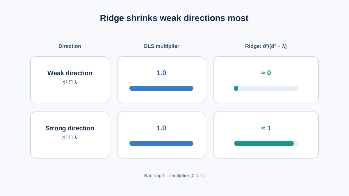
Each direction gets multiplied by the factor $\frac{d_j^2}{d_j^2 + \lambda}$. That factor is the whole mechanism. It is always between 0 and 1, so every direction is shrunk. But the amount depends on $d_j$.

• Directions with large singular values — strong, well-determined directions — have $d_j^2 \gg \lambda$, so the factor is close to 1. They barely move.
• Directions with small singular values — the collinear, unstable directions — have $d_j^2 \ll \lambda$, so the factor is close to 0. They get crushed.

This is why ridge handles multicollinearity so well. The directions that OLS amplifies into wild coefficients are exactly the directions ridge shrinks hardest. The penalty is not applied uniformly; it is applied where the data is weakest.

The tradeoff is bias for variance. Ridge introduces bias because it pulls coefficients away from their OLS values. In exchange, it reduces the variance of the estimates, because small perturbations in the data no longer produce large swings in the coefficients. Whether the net effect on expected test error is positive depends on $\lambda$. Choose it badly and you get more bias than the variance reduction is worth.

One behavioral note that separates ridge from lasso: ridge shrinks coefficients toward zero but never sets them exactly to zero. The penalty is smooth and differentiable at zero, so the minimum is generically not at zero. Lasso uses an absolute-value penalty, which has a kink at zero, and that kink is what produces exact zeros and feature selection.

Finally, the penalty is not scale-invariant. It penalizes the raw magnitude of each coefficient. A feature measured in small units gets a large coefficient, and ridge punishes it harder than a feature measured in large units — for no statistical reason. Standardize your features before fitting.

A Small Worked Example

Numbers make the shrinkage visible. Take a tiny dataset with two nearly identical features.

$X = \begin{bmatrix} 1 & 1.01 \\ 2 & 1.99 \\ 3 & 3.02 \\ 4 & 3.98 \end{bmatrix}, \qquad y = \begin{bmatrix} 1 \\ 2 \\ 3 \\ 4 \end{bmatrix}$

The two columns are almost the same feature. Compute $X^\top X$:

$X^\top X = \begin{bmatrix} 30 & 30.02 \\ 30.02 & 30.05 \end{bmatrix}$

The determinant is $30 \times 30.05 - 30.02^2 \approx 901.5 - 901.2 = 0.3$. A matrix with entries around 30 and a determinant of 0.3 is nearly singular. Now compute $X^\top y \approx (30, 30.04)^\top$ and solve the normal equations. The OLS coefficients come out approximately:

$\hat{\beta}_{\text{OLS}} \approx (0.5, 0.5)$

Wait — that looks tame. Try a slightly different target, $y = (1, 2, 3, 4.1)^\top$. The tiny change in the last entry flips the solution to roughly:

$\hat{\beta}_{\text{OLS}} \approx (-4.5, 5.5)$

The coefficients exploded. The predictions barely changed, because $-4.5 \times x_1 + 5.5 \times x_2 \approx 0.5 x_1 + 0.5 x_2$ when $x_1 \approx x_2$. This is the instability in its purest form.

Now apply ridge. For each $\lambda$, compute $(X^\top X + \lambda I)^{-1} X^\top y$:

Watch what happens. At $\lambda = 1$, the coefficients have already shrunk dramatically. At $\lambda = 10$, they are close to the stable $(0.5, 0.5)$ solution. At $\lambda = 100$, they are nearly equal and small.

The predictions move far less than the coefficients. At $\lambda = 0$, the prediction for the first row is $-4.5 + 5.5 \times 1.01 \approx 1.06$. At $\lambda = 10$, it is $0.1 + 0.9 \times 1.01 \approx 1.01$. The fit is nearly preserved while the coefficient vector is tamed. That is the tradeoff in one table.

You can verify the closed form against scikit-learn with a few lines:

import numpy as np
from sklearn.linear_model import Ridge

X = np.array([[1, 1.01], [2, 1.99], [3, 3.02], [4, 3.98]])
y = np.array([1, 2, 3, 4.1])

# Closed form
for lam in [0, 1, 10, 100]:
    beta = np.linalg.solve(X.T @ X + lam * np.eye(2), X.T @ y)
    print(f"lambda={lam:>3}: {beta.round(3)}")

# Library check (fit_intercept=False to match the derivation)
for lam in [1, 10, 100]:
    model = Ridge(alpha=lam, fit_intercept=False).fit(X, y)
    print(f"sklearn alpha={lam:>3}: {model.coef_.round(3)}")

The closed form and the library result match. That is the point of deriving it: you can predict the output before you run the code.

Choosing λ and Knowing the Limits

The derivation gives you the solution for any fixed $\lambda$. It does not tell you which $\lambda$ to use. That is a hyperparameter, selected by cross-validation, not derived in closed form. Fit ridge across a grid of $\lambda$ values, evaluate each on held-out folds, and pick the one with the best validation error.

A few practical rules:

• Standardize features first. The penalty is not scale-invariant. Without standardization, ridge penalizes features unevenly for reasons that have nothing to do with their predictive value.
• Do not penalize the intercept. Center your data or exclude the intercept from the penalty. Penalizing it biases predictions away from the target mean.
• Know the boundaries. Ridge assumes a linear model with squared-error loss. It shrinks coefficients but never sets them to zero, so it does not perform feature selection. If you need sparse coefficients, an L1 penalty is the right tool.
• When to reach for ridge first. If your features are correlated, if $p$ is close to or larger than $n$, or if OLS coefficients look unstable across resamples, ridge is the principled first move. If you need interpretability through feature elimination, or if you have strong reason to believe only a few features matter, consider lasso instead.

The penalty is not a hack bolted onto least squares. It is the mathematically clean way to restore a unique, stable solution when the normal equations cannot provide one.

Your next step: take a dataset you already have, standardize the features, and fit both OLS and ridge across a small grid of $\lambda$ values. Print the coefficient vectors side by side. When you see the coefficients settle down while the predictions hold steady, you will have watched the derivation do its job.