Build a Sparse-Text Naive Bayes Classifier With Scikit-Learn

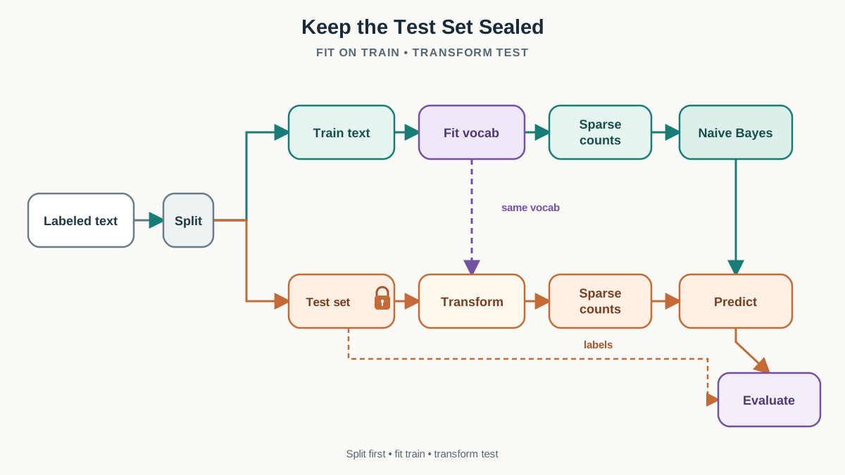
The most dangerous bug in a beginner text classifier is not in the model. It is in the order of operations. Fit your vectorizer on the whole dataset before splitting, and you will get a score that looks excellent and means almost nothing.

We are going to build the workflow that prevents that by construction: split first, learn the vocabulary from training text only, fit a Naive Bayes model, inspect real predictions, and then test how the representation changes the result. Everything runs on a laptop in seconds.

What You Are Building and Why Naive Bayes Fits Text

Naive Bayes multiplies per-feature evidence together under an independence assumption: it treats each token as a separate vote for a class. Text is a natural fit because most documents contain only a small fraction of the full vocabulary, so the feature matrix is sparse — mostly zeros, and the zeros are never stored.

The task here is a small labeled text dataset with a handful of classes, split into train and test. For word-count features, MultinomialNB is the default choice. Reach for BernoulliNB when you care about presence versus absence of tokens rather than counts, and ComplementNB when classes are imbalanced.

You need Python with scikit-learn, NumPy, and pandas. No GPU, no external services.

Success looks like this: a fitted model, a test score, and a readable table of predictions with probabilities you can actually interpret.

Load the Data and Split Before You Touch the Text

Start with labels and raw text in a DataFrame. Print the shape and a couple of rows so you see what the model will consume.

import pandas as pd
from sklearn.model_selection import train_test_split

df = pd.DataFrame({
    "text": [
        "the team won the match in extra time",
        "new phone update fixes the battery drain",
        "election results spark debate in parliament",
        "the striker scored twice in the final",
        "chip maker announces faster processor",
        "senate passes the new budget bill",
        "coach praises defense after the win",
        "software release adds dark mode",
        "minister resigns after the vote",
        "league standings tighten after weekend games",
    ],
    "label": [
        "sports", "tech", "politics",
        "sports", "tech", "politics",
        "sports", "tech", "politics", "sports",
    ],
})

X_train, X_test, y_train, y_test = train_test_split(
    df["text"], df["label"], test_size=0.3, random_state=42, stratify=df["label"]
)

The random_state makes the split reproducible. The stratify argument keeps the class proportions balanced across both sides.

Here is the rule that the rest of this tutorial depends on: the test set is sealed until the final evaluation. Any vocabulary, token statistic, or class balance you learn from it is leakage.

This matters more for text than for numeric features because the vocabulary itself is learned from data. If the vectorizer sees test documents while building its word list, the model already knows which words exist in the exam it is about to take.

Common mistake: calling fit_transform on the full corpus and then splitting. The score goes up, and the number becomes fiction.

Turn Text Into a Sparse Count Matrix

CountVectorizer learns a vocabulary on the training text, then maps documents to token counts. It is a fitted transformation, not a pure function.

from sklearn.feature_extraction.text import CountVectorizer

vectorizer = CountVectorizer(lowercase=True, stop_words="english")
X_train_counts = vectorizer.fit_transform(X_train)
X_test_counts = vectorizer.transform(X_test)

print(X_train_counts.shape)
print(X_train_counts.nnz)  # number of non-zero entries

Notice the asymmetry: fit_transform on train, transform on test. Swap them and the test vocabulary leaks into training. Fit on test and you have trained on the exam.

The shape tells you documents by vocabulary size. The nnz count tells you how many entries are actually stored. If you stored every zero, a modest corpus would balloon into a dense array of mostly nothing.

To connect a row of numbers back to words:

feature_names = vectorizer.get_feature_names_out()
row = X_train_counts[0].toarray().ravel()
for i in row.nonzero()[0]:
    print(feature_names[i], row[i])

A few practical knobs change the vocabulary size directly: lowercase, stop_words, ngram_range, min_df (drop terms appearing in fewer than N documents), and max_df (drop terms appearing in more than a fraction of documents).

Failure signal: a vocabulary that is huge and mostly noise, or a test document with zero known tokens. Both mean your representation is not carrying signal.

Fit MultinomialNB and Read the Predictions

Now fit the model on the training counts and labels.

from sklearn.naive_bayes import MultinomialNB

model = MultinomialNB(alpha=1.0)
model.fit(X_train_counts, y_train)

preds = model.predict(X_test_counts)
probs = model.predict_proba(X_test_counts)

alpha is the smoothing parameter and defaults to 1.0. It adds a small count to every feature so that a single unseen word cannot zero out an entire class.

Do not stop at the score. Inspect the output:

import numpy as np

for text, true, pred, prob in zip(X_test, y_test, preds, probs):
    confidence = prob.max()
    print(f"{true:>9} -> {pred:<9} ({confidence:.2f})  {text[:40]}")

predict_proba returns a distribution over classes, not just a winner. These are not calibrated probabilities — a 0.95 does not mean the model is right 95% of the time. Treat them as relative confidence.

To see which tokens push a class up or down, inspect feature_log_prob_ and class_log_prior_. This connects directly back to the mechanism: the model multiplies evidence per token, so a token with high log-probability for a class acts as a strong vote.

Failure mode: a confident wrong prediction on a short document. Smoothing keeps any single unseen word from zeroing out a class, but it cannot rescue a document with almost no signal.

Evaluate Honestly and Watch for the Leakage Tell

Report accuracy alongside a confusion matrix so per-class failures are visible instead of hidden in one number.

from sklearn.metrics import accuracy_score, confusion_matrix

print(accuracy_score(y_test, preds))
print(confusion_matrix(y_test, preds, labels=model.classes_))

Now run the broken version deliberately. The key is to reuse the exact same train/test rows so the only thing that changes is the vectorizer's information boundary:

from sklearn.model_selection import train_test_split

# Recreate the identical split indices
idx_train, idx_test = train_test_split(
    df.index, test_size=0.3, random_state=42, stratify=df["label"]
)

# Broken: vectorizer sees all text before the split
leaky_vec = CountVectorizer(stop_words="english")
X_all = leaky_vec.fit_transform(df["text"])

Xtr_leak = X_all[idx_train]
Xte_leak = X_all[idx_test]
ytr_leak = df["label"].iloc[idx_train]
yte_leak = df["label"].iloc[idx_test]

leaky_model = MultinomialNB().fit(Xtr_leak, ytr_leak)
print(accuracy_score(yte_leak, leaky_model.predict(Xte_leak)))

The scores may or may not differ on ten examples. That is the point: do not trust a score gap as proof of leakage. The real evidence is in the vocabulary. Compare the two vocabularies directly:

print("Clean vocab size:", len(vectorizer.get_feature_names_out()))
print("Leaky vocab size:", len(leaky_vec.get_feature_names_out()))

clean_vocab = set(vectorizer.get_feature_names_out())
leaky_vocab = set(leaky_vec.get_feature_names_out())
test_only_words = leaky_vocab - clean_vocab
print("Words the leaky vectorizer saw only in test:", test_only_words)

Any word in test_only_words is vocabulary the model should not have known about. That is the leakage tell — a vocabulary boundary violation, not a suspiciously high score.

Note: accuracy alone misleads when one class dominates. Macro-averaged precision and recall are the next step, but keep the evaluation small and honest rather than adding cross-validation machinery you have not met yet.

Change the Representation and Watch the Score Move

Naive Bayes treats tokens as independent evidence, so repeated or correlated words get double-counted. That is why representation changes move the result.

Experiment 1: TF-IDF instead of raw counts.

from sklearn.feature_extraction.text import TfidfVectorizer

tfidf = TfidfVectorizer(stop_words="english")
Xtr_tfidf = tfidf.fit_transform(X_train)
Xte_tfidf = tfidf.transform(X_test)
tfidf_model = MultinomialNB().fit(Xtr_tfidf, y_train)
print(confusion_matrix(y_test, tfidf_model.predict(Xte_tfidf), labels=tfidf_model.classes_))

Compare the confusion matrices, not just the accuracy.

Experiment 2: add bigrams.

bigram_vec = CountVectorizer(ngram_range=(1, 2), stop_words="english")
Xtr_bi = bigram_vec.fit_transform(X_train)
Xte_bi = bigram_vec.transform(X_test)
print(bigram_vec.get_feature_names_out().shape)

Watch the vocabulary grow and the errors shift.

Experiment 3: vary alpha.

for a in [0.01, 0.1, 1.0, 10.0]:
    m = MultinomialNB(alpha=a).fit(X_train_counts, y_train)
    print(a, accuracy_score(y_test, m.predict(X_test_counts)))

Smoothing is a real tradeoff, not a formality.

Experiment 4: make the independence assumption visible.

The independence assumption says each token contributes evidence on its own. When two words always appear together, the model counts that evidence twice. You can observe this directly by duplicating a token in the text and watching the class probability shift:

# Take one test document and duplicate a word that appears in it
sample = X_test.iloc[0]
print("Original:", sample)

# Manually duplicate a token by editing the raw text
words = sample.split()
if len(words) > 1:
    doubled = sample + " " + words[1]  # repeat the second word
    print("Doubled:", doubled)

    # Vectorize both and compare probabilities
    orig_vec = vectorizer.transform([sample])
    doubled_vec = vectorizer.transform([doubled])
    print("Original probs:", model.predict_proba(orig_vec)[0])
    print("Doubled probs: ", model.predict_proba(doubled_vec)[0])

The probability shifts because the repeated word acts as two independent votes for the same class. In real text, correlated words like "New" and "York" or "machine" and "learning" do this constantly. The model cannot tell that they are one piece of evidence, not two.

Decision rule: if a linear model with TF-IDF clearly beats Naive Bayes on the same split, that is a signal to move on, not a reason to keep tuning.

Wrap It in a Pipeline So the Order Cannot Break

Manual steps work, but they rely on you remembering the order. A pipeline enforces it by construction.

from sklearn.pipeline import Pipeline

pipe = Pipeline([
    ("vec", CountVectorizer(stop_words="english")),
    ("nb", MultinomialNB(alpha=1.0)),
])

pipe.fit(X_train, y_train)
print(accuracy_score(y_test, pipe.predict(X_test)))

This reproduces the manual result. The real payoff is that leakage becomes structurally harder: the vectorizer only ever sees the data passed to fit, and the same object is what you would hand to cross-validation or save to disk.

The same pipeline shape transfers to other sparse-text classifiers. Swap the final step and keep the workflow.

Where This Breaks and What to Try Next

The independence assumption is false for natural language. Probabilities are not calibrated. Very short documents give unstable estimates. These are real limits, not footnotes.

Naive Bayes is the right first move when you have a small labeled dataset, many sparse features, and you want a fast interpretable baseline you can beat later. Reach for something else when feature interactions matter, when you need long-range context, or when you need calibrated probabilities.

Your next step: take the exact pipeline above, swap MultinomialNB for a linear model with TF-IDF, and compare confusion matrices on the identical split. Same data, same split, different model. The errors will tell you which one actually understands your text.