
Why Lasso Can Set Coefficients to Zero: An L1 Derivation
Fit a lasso on a dataset with a dozen features and something strange happens. A few coefficients come back as exactly 0.0. Not 0.0031. Not 0.0007. Zero.…

Key topics
Fit a lasso on a dataset with a dozen features and something strange happens. A few coefficients come back as exactly 0.0. Not 0.0031. Not 0.0007. Zero. Fit ridge on the same data and every coefficient survives, small but alive.
The usual explanation — "the penalty pushes small numbers down until they round to zero" — is wrong, and it hides the actual mechanism. Nothing is rounding. The optimizer is choosing a point where a coefficient is exactly zero because that point is genuinely optimal under the L1 penalty. To see why, we need the objective, the constraint geometry, and one small case where you can watch a coefficient cross the line.
This is the derivation. I'll assume you already have OLS normal equations and ridge shrinkage in hand — if not, the prerequisite articles cover both. Here we start from the lasso objective and follow it to the zero.
Set Up the Objective and the Notation
Fix the notation first, because every later symbol needs a concrete referent.
Let be the design matrix — observations, features. Let be the -vector of targets. Let be the -vector of coefficients we are solving for. The residual vector is
The intercept is handled separately and is not penalized. Penalizing it would make the fit depend on where you happened to center the target, which is not a modeling choice you want the penalty making for you.
The lasso objective is
Read it term by term:
- is the squared error — the fit term. It wants to explain the data.
- is the L1 norm — the penalty term. It wants to be small, and it charges for every nonzero entry.
- is the single knob trading one against the other.
Ridge uses the same framework with one structural change: the penalty becomes . Same fit term, same , different norm. That single substitution is the entire source of the behavioral difference, and the rest of this article is about why.
Three assumptions carry the derivation:
- Columns of are standardized (centered and scaled to unit variance). The L1 penalty charges absolute magnitude, so if one feature is measured in millimeters and another in kilometers, you are penalizing units, not signal.
- . A negative penalty would reward large coefficients, which is not regularization.
- No perfect collinearity in , so the solution is unique.
Knowledge check
Check your understanding
Answer this question before you continue.
Two Equivalent Views: Penalty and Constraint
The penalized form above is convenient for computation. The constrained form is convenient for geometry, and they describe the same solution set.
For every there exists some that yields the same solution, and vice versa. This is Lagrangian duality — I am stating it, not proving it here. The practical content is the direction of the knob: larger corresponds to smaller , which means more shrinkage and more zeros.
Now picture the two pieces.
The squared-error term draws ellipsoids around the OLS solution . Each ellipsoid is a contour of equal error: points on the same ellipse fit the data equally well. The center is , the unpenalized optimum.
The constraint draws a region around the origin. For L1 that region is a diamond in two dimensions; for L2 it is a circle.
The lasso solution is the first point where a growing error ellipsoid touches the constraint region. Start with a tiny ellipsoid near — it misses the constraint entirely. Inflate it. The moment it makes contact, you have found the constrained optimum. That contact point is the answer.
Everything that follows is about the shape of the thing the ellipsoid touches.
Knowledge check
Check your understanding
Answer this question before you continue.
Why the Diamond Has Corners and the Circle Does Not
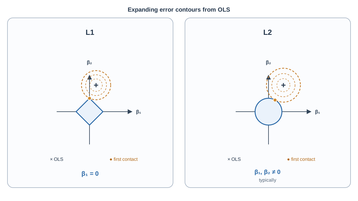
In two dimensions, the L1 ball is a diamond with vertices sitting on the axes at , , , and . In dimensions it becomes a cross-polytope, and its vertices and low-dimensional faces lie on coordinate subspaces — places where one or more coefficients are exactly zero.
The L2 ball is a smooth sphere. No vertices. No flat faces. Its boundary curves everywhere, so an expanding ellipsoid generically meets it at a single tangent point in the interior of a face — a spot where every coordinate is nonzero. Coordinate-zero points do exist on the sphere (the axis points), but the smooth boundary gives the ellipsoid no reason to prefer them.
Here is the touch argument. An expanding ellipsoid generically first contacts a smooth surface at a tangent point in the interior of a face — a spot where every coordinate is nonzero. It can contact a corner exactly, and corners sit where some .
Be honest about the word "generically." The corner is not guaranteed. But it is a positive-probability event for L1 and a measure-zero event for L2. That asymmetry is the whole story: the diamond offers the ellipsoid a set of zero-coordinate landing pads, and the circle offers none.
Note: The corner is not the only way to get a zero. In higher dimensions the ellipsoid can land on an edge or a face of the cross-polytope, and any such contact pins at least one coefficient to zero. The vertex is just the easiest picture to hold in your head.
The Coordinate-Wise View: Soft Thresholding
The geometry is convincing, but I do not want you to take sparsity on faith from a picture. There is a second route to the same conclusion, and it is algebraic.
Take the special case where the design is orthonormal: . This is a teaching device, not the general case, but it strips the problem down to its mechanism. Under orthonormality the lasso solution reduces to
Read that as a mechanism, not a formula. Take the OLS coefficient. Subtract from its magnitude. If nothing is left, the coefficient is exactly zero — not small, zero. This is soft thresholding, and it is the cleanest statement of lasso coefficient thresholding:
Compare ridge under the same orthonormal design:
Ridge divides. Lasso subtracts. Division by a finite number never reaches zero, no matter how large grows. Subtraction crosses zero and stops there. That is the difference between shrinkage and selection, and it is the same fact the diamond was showing you.
Common mistake: Treating the orthonormal result as the general rule. With correlated predictors, the threshold is no longer a clean per-coefficient comparison against . The next section shows what actually happens.
Knowledge check
Check your understanding
Answer this question before you continue.
A Small Worked Case: Shrinkage, Then a Zero
Let's make it concrete. Two standardized predictors, and suppose the OLS solution is
I am choosing these numbers so the arithmetic stays hand-checkable. In the orthonormal case, soft thresholding gives the lasso solution directly:
Walk upward and watch what happens.
| 0.0 | 2.0 | 0.5 |
| 0.2 | 1.8 | 0.3 |
| 0.5 | 1.5 | 0.0 |
| 1.0 | 1.0 | 0.0 |
| 2.0 | 0.0 | 0.0 |
At the second coefficient hits zero, because . The threshold condition is satisfied exactly, and the coefficient does not pass through zero into negative territory — it stops. For any , feature 2 is gone from the model. At , feature 1 follows.
That moment at is what "selection" means operationally: the active feature set changes. Before it, two features carry weight. After it, one does. The model did not merely get smaller; its structure changed.
One more piece of context worth knowing: the full solution path is piecewise linear in . Between threshold crossings, each coefficient moves along a straight line. That is why path algorithms can compute the entire sequence of solutions efficiently rather than refitting from scratch at every — but that is an implementation detail, not part of the derivation.
Knowledge check
Check your understanding
Answer this question before you continue.
What the Derivation Does Not Promise
A zero coefficient is a statement about the objective at a particular . It is not a statement about the world. Five limits matter.
Correlated predictors. With near-duplicate columns, lasso tends to keep one and zero the other, and which one it picks can flip across resamples. The predictions may be stable while the selection is not. If your features come in correlated groups, this instability is the norm, not an edge case.
Sparse is not important. A zero means "this coefficient was not worth its L1 cost at this ." It does not mean the variable is irrelevant. A feature can be genuinely predictive and still be zeroed because a correlated neighbor already carries the signal.
Scaling matters. Penalizing raw coefficients on unstandardized features penalizes measurement units. Standardize first, or the penalty is doing something you did not intend.
Recovery has conditions. Exact support recovery — getting the true nonzero set back — requires enough samples, low noise, and a design that is not too correlated. When those conditions fail, L1 selection can behave close to random. The number of samples needs to be sufficiently large relative to the number of true nonzero coefficients, the noise level, and the correlation structure of .
is a modeling decision. Cross-validation tends to under-penalize, keeping a few irrelevant features because they do not hurt prediction. BIC-style criteria tend to over-penalize. Neither is a truth oracle; they optimize different things.
When to Reach for Lasso, and When Not To
Convert the mechanism into a decision rule.
Reach for lasso when is large relative to , you suspect only a subset of features matter, and you want a sparse, inspectable model. The corners of the L1 ball are doing useful work for you.
Prefer ridge when predictors are many and correlated and you mainly care about prediction stability rather than selection. Ridge will not hand you a feature list, but it will not hand you an unstable one either.
Consider elastic net when you want sparsity but need correlated groups to enter or leave together. It blends the L1 and L2 penalties, which is the natural extension when the diamond's corners are too sharp for your data.
And do not treat a lasso fit as a causal or scientific conclusion. Treat it as a hypothesis generator. The zero coefficients tell you which features might deserve attention; held-out validation tells you whether that attention pays off.
Tip: Put scaling and the penalty inside a pipeline so the same transformation is applied at fit and predict time. A scaler fitted on training data and forgotten at prediction time is a quiet, recurring bug.
Where to Go Next
The zero coefficients come from the corners of the L1 ball, and the soft-thresholding formula is the same fact written in algebra. Two views, one mechanism.
Here is the next move I would make. Take a small standardized dataset, fit a lasso, and sweep across a wide range. Plot the coefficient path — on a log scale against each coefficient. Watch a line dive to zero and stay there. That picture will do more for your intuition than any derivation, because you will have produced it yourself.
Then apply the decision rule: use the sparsity as a hypothesis about which features deserve attention, and verify it out of sample before you believe it.
Knowledge check
Final check
Finish the article by checking the ideas you just learned.
References
Build stronger machine learning foundations
Use structured resources to connect theory, scikit-learn workflows, and evaluation practice.


