
Regularization in Machine Learning: Ridge, Lasso, and Simpler Models
Regularization is not a magic switch that makes every model better. It is a deliberate trade: you give up a little accuracy on your training data to gain…

Key topics
Regularization is not a magic switch that makes every model better. It is a deliberate trade: you give up a little accuracy on your training data to gain stability on data the model has never seen.
If you have trained a few linear models, you have probably seen the pattern. The training error looks great. The validation error tells a different story. The gap between those two numbers is the symptom of overfitting, and large, unstable coefficients are part of the mechanism. When a model must assign a huge weight to one feature just to accommodate a single noisy point, it is contorting itself to the training data rather than describing a real pattern.
Regularization in machine learning addresses that mechanism directly. It adds a constraint that keeps coefficients from growing too large, forcing the model to find a simpler explanation for the data. The result is usually a model that generalizes better, but only if you understand what the penalty is actually doing.
Why a Perfect Fit Is Not the Goal
A model that fits training data perfectly has often memorized noise. Think about what a large coefficient means: the model's prediction swings wildly when that feature changes by even a small amount. That sensitivity is rarely justified by the underlying pattern. More often, it exists because the model discovered that a particular training point could be nailed more precisely if one feature was allowed to dominate.
The fix is not to find a model that fits harder. It is to constrain how far the coefficients can travel in pursuit of a perfect training score. Regularization imposes exactly that constraint. It trades a small amount of training accuracy for a model whose predictions depend less on the specific accidents of your training sample.
That trade is the entire game. You are not looking for the model with the lowest training error. You are looking for the model that will behave well when it meets new data.
The Regularized Objective: Fitting with a Hand Brake
Recall the least-squares objective from linear regression: minimize the sum of squared differences between predictions and actual values. The model finds coefficients that make that sum as small as possible.
Regularization adds a second term to that objective. The new loss function looks like this:
Loss = Fit to training data + α × Penalty on coefficient size
The fit term is the familiar prediction error. The penalty term is new. It grows as coefficients grow, which means the model now has two competing goals: fit the data well, and keep coefficients small. The parameter α (sometimes called lambda) controls how much weight the penalty carries.
One detail matters before we go further: the penalty applies to the feature coefficients, not the intercept. The intercept just shifts predictions up or down to match the target's average, so letting it grow large does not create the same overfitting risk. When you see the penalty written as a sum over coefficients, it is a sum over the features.
Here is what α does in plain terms:
- Small α: The penalty barely matters. The model behaves almost like unregularized least squares and can still overfit.
- Large α: The penalty dominates. Coefficients are pushed hard toward zero, and the model may become too simple to capture real patterns.
The observable signal is clear. As α rises, coefficients shrink, and training error rises. Validation error often falls first, then rises again as the penalty becomes too aggressive. That U-shape in validation error is the bias-variance trade playing out in front of you.
The ideal α is data-dependent. There is no universal default that works for every problem, which means you will tune it with validation data rather than assuming a value.
Knowledge check
Check your understanding
Answer this question before you continue.
Ridge (L2): Shrink Everything, Keep Everything
Ridge regression uses an L2 penalty, which sums the squares of the coefficients:
Penalty = β₁² + β₂² + ... + βₚ²
Because the penalty squares each coefficient, large values are punished disproportionately. A coefficient of 5 contributes 25 to the penalty; a coefficient of 0.5 contributes only 0.25. The model learns that letting any single feature grow very large is expensive, so it spreads influence more evenly across features.
The key behavior of ridge: coefficients shrink toward zero, but they rarely reach it. Every feature keeps at least a small voice in the prediction. When you have correlated features, ridge tends to share weight among them rather than picking a favorite. That makes ridge a strong default when your main goal is prediction stability and you have no strong reason to believe most features are useless.
If you plot ridge coefficients against α, you will see them collapse toward zero as the penalty grows. The general pattern is clear: higher α means smaller coefficients, and the features that needed the largest values to fit noise are the ones that lose the most influence.
Knowledge check
Check your understanding
Answer this question before you continue.
Lasso (L1): Shrink and Select
Lasso uses an L1 penalty, which sums the absolute values of the coefficients:
Penalty = |β₁| + |β₂| + ... + |βₚ|
That small change from squaring to absolute value produces a dramatically different behavior. Under the L1 penalty, some coefficients are driven exactly to zero. The model removes those features entirely.
This makes lasso a feature selector as much as a regularizer. When a sparse feature representation is operationally useful, lasso will zero out features and leave you with a model that is easier to read. You can look at the remaining coefficients and say, "these are the features the model kept."
The tradeoff appears with correlated features. Where ridge shares weight across correlated predictors, lasso tends to pick one and discard the others. That can be useful for interpretability, but it can also be unstable: a slightly different training sample might cause lasso to choose a different feature from the correlated group.
Common mistake: A lasso coefficient of exactly zero does not prove the feature is unimportant. It may simply mean the feature is correlated with another feature that lasso chose to keep. The discarded feature might carry real predictive signal; lasso just decided it was redundant. Sparse is not the same as scientifically meaningful.
One practical note: neither ridge nor lasso is scale-invariant. If one feature is measured in dollars and another in thousands of dollars, the penalty will treat them unfairly. Scale your features before applying either penalty.
Knowledge check
Check your understanding
Answer this question before you continue.
Ridge vs Lasso: A Comparison Table
| Dimension | Ridge (L2) | Lasso (L1) |
|---|---|---|
| Penalty form | Sum of squared coefficients | Sum of absolute coefficients |
| Effect on coefficients | Shrinks toward zero | Shrinks toward zero |
| Reaches exactly zero | Rarely | Often |
| Feature selection | No | Yes |
| Correlated features | Shares weight among them | Picks one, ignores others |
| Best when | Prediction stability matters and features carry overlapping signal | A sparse, readable model is operationally valuable |
| Primary goal | Stable predictions with all features retained | Sparse model with fewer features |
Both require feature scaling. Both require tuning α. The choice between them is not about which is more advanced or more correct. It is about what your modeling problem demands.
Choosing a Penalty from the Problem, Not a Slogan
Beginners often ask which regularization technique is best, as if the answer were a fixed preference. It is not. The right question is what your model is for.
Start with ridge when: you have many features that plausibly contribute to the prediction, you have correlated predictors, and your main goal is prediction quality. Ridge will stabilize the model without forcing you to discard information, and it will not make arbitrary choices among correlated features.
Try lasso when: a sparse feature representation is genuinely useful for your workflow, and you can tolerate some instability in which features get selected. Lasso will make the feature selection decision for you, which is valuable when interpretability matters more than squeezing out the last bit of prediction accuracy.
Use neither when: a simpler model or careful feature engineering would serve you better. Regularization is not a substitute for understanding your data. If you have a small number of meaningful features and no overfitting problem, adding a penalty just introduces bias without buying stability.
The common mistake is treating regularization as a default that always helps. It does not. Crank α too high and you will underfit, producing a model too simple to capture the real pattern. The penalty is a tool for controlling complexity, not an automatic improvement.
Knowledge check
Check your understanding
Answer this question before you continue.
Tuning α Without Fooling Yourself
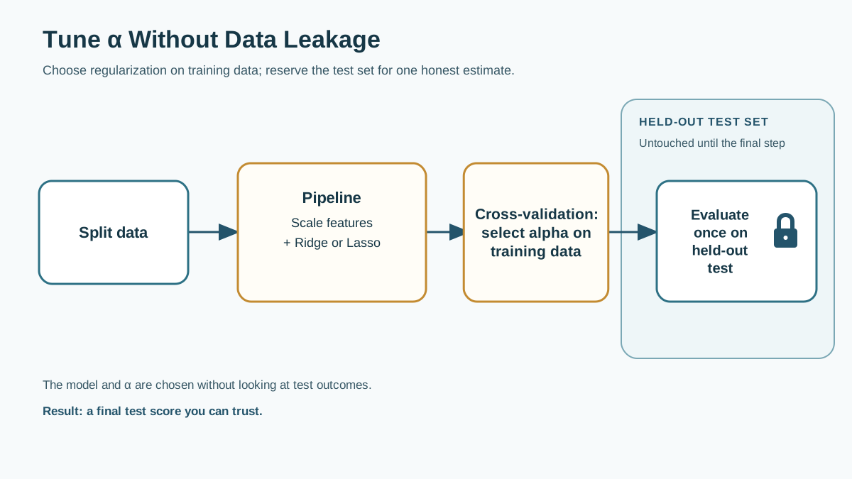
The way you choose α matters as much as the penalty itself. A sloppy tuning workflow can produce an optimistic performance estimate that falls apart when the model meets new data.
Here is the workflow I recommend:
- Split off a final test set first. Set aside a portion of your data and do not touch it until the very end. This is your honest estimate of how the model will behave on new data.
- Put scaling and the model in a pipeline. Standardize features and fit Ridge or Lasso inside a scikit-learn
Pipeline. This prevents a subtle but common leak: scaling on the full dataset before splitting lets information from the test set influence training. - Choose α with cross-validation on the training portion. Use
GridSearchCVorRidgeCV/LassoCVto search over α values. Cross-validation repeatedly splits the training data into smaller training and validation folds, so every candidate α gets tested on data it did not see during fitting. - Evaluate the chosen model on the untouched test set once. That single number is your realistic estimate of generalization. If you use the test set repeatedly to make modeling decisions, it stops being an honest test.
Warning: Tuning α on the training set will always pick a very small penalty, because the unregularized model fits training data best. That defeats the purpose. The whole point of the penalty is to sacrifice a little training fit for better behavior on unseen data, and you can only measure that behavior on data the model did not train on.
Common Mistakes and Practical Checks
A few errors show up repeatedly when people start using regularization.
Forgetting to scale features. The penalty assumes all features live on comparable scales. If one feature has values in the thousands and another in the hundredths, the penalty will hammer the small-scale feature into irrelevance regardless of its true importance. Scale first, then regularize.
Misreading zeroed lasso coefficients. As noted above, a zero does not mean "no predictive information." It means "not needed given the other features in the model." Check whether the zeroed feature is correlated with a survivor before drawing conclusions.
Ignoring the validation curve. The most informative plot in regularization is validation error against α. Watch it as α increases. If validation error falls, you were overfitting and the penalty is helping. If validation error rises immediately, you were not overfitting, and the penalty is only adding bias.
Choosing the sparsest model instead of the best model. Lasso can zero out many features at high α, and a sparse model can look elegant. But elegance is not the goal. The goal is the α that minimizes validation error. If the sparsest model performs worse on held-out data, the extra zeros cost you real prediction quality.
The Experiment That Makes It Click
The fastest way to internalize regularization machine learning is to run a small comparison on the same dataset. Fit an unregularized linear model, a ridge model, and a lasso model. Plot the coefficients against α for the regularized models and watch them shrink. Then plot the validation curve and watch it fall, bottom out, and rise again.
Before you run it, know what you are looking for:
- Ridge coefficients should shrink smoothly toward zero as α rises, but most should stay nonzero even at large penalties.
- Lasso coefficients should start dropping to exactly zero one by one as α rises, leaving a visibly sparse set of survivors.
- Validation error should improve as α rises from zero, then worsen once the penalty grows too strong. The best α is the bottom of that curve, not the point where the model looks simplest.
That single experiment shows you the whole trade in action: coefficients collapsing, training error climbing, validation error improving until the penalty becomes too strong. After you have seen that curve once, regularization stops being an abstract concept and becomes a lever you know how to pull.
Choose the penalty from the modeling problem. Tune α with cross-validation inside a pipeline. Judge the result on a test set you touched only once. And remember that regularization is one tool among several for controlling complexity, not a replacement for understanding your data.
Knowledge check
Final check
Finish the article by checking the ideas you just learned.
References
Research updated Sep 8, 2026


