Compare Random, Grouped, and Time-Based Validation in Scikit-Learn

Same model. Same features. Two validation schemes. One score says 0.94, the other says 0.61.

The first time I watched that gap appear, I assumed I had broken something. I hadn't. The model was fine. The random split was answering a question nobody would ever ask.

Here is the mental model that fixes this: a validation split is not a way to hold data back. It is a simulation of deployment. When you call train_test_split, you are asserting that a held-out row is exchangeable with a training row — that knowing one tells you nothing about the other. Statisticians call this the i.i.d. assumption. In operational terms, it means the future looks like a shuffled version of the past.

When rows share an entity — the same user, patient, store, or device — or when they carry a time order, that assertion is false. The split quietly grades the model on rows it has effectively already seen. The score is not lying. It is answering exactly what you asked. You asked the wrong question.

This article assumes you already know why ordinary folds can be invalid. We are going to measure how much the answer changes, and why. Two dependence structures, three splitters, one side-by-side table.

What a Split Is Actually Claiming

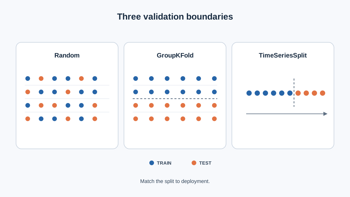
Before the code, name the two structures we will use.

Repeated entities (grouped). Each entity contributes several rows. If entity identity influences the target, a random split scatters near-duplicates across both sides of the boundary, and the model gets partial credit for memorizing the entity rather than learning the signal.

Temporal ordering (time-based). Rows are generated in sequence, and later rows are not drawn from the same distribution as earlier ones. A random split lets the model train on the future and predict the past — a task that never exists in production.

Both cases break the same assumption. Both produce the same symptom: a score that looks like success and means nothing.

Build the Two Datasets

Everything below runs on scikit-learn, NumPy, and pandas. No downloads, no credentials, fixed seed, a few hundred rows. Run it and confirm the shapes before you trust a single score.

The critical design choice is that the model must be able to see the structure we are testing. If the group identifier or time index never reaches the features, the model cannot exploit the dependence, and the experiment proves nothing. So we expose both.

import numpy as np
import pandas as pd
from sklearn.ensemble import RandomForestRegressor
from sklearn.model_selection import (
    train_test_split, cross_val_score, GroupKFold, TimeSeriesSplit
)

rng = np.random.default_rng(0)

# Dataset A — grouped: 40 entities x 8 rows each
n_entities, rows_per_entity = 40, 8
entity_id = np.repeat(np.arange(n_entities), rows_per_entity)
entity_effect = rng.normal(0, 5, n_entities)[entity_id]   # strong entity signal
x1 = rng.normal(0, 1, entity_id.size)
x2 = rng.normal(0, 1, entity_id.size)
y_grouped = entity_effect + 0.5 * x1 + rng.normal(0, 0.5, entity_id.size)

df_grouped = pd.DataFrame(
    {"entity": entity_id, "x1": x1, "x2": x2, "y": y_grouped}
)

# Dataset B — temporal: drift over time
n = 300
t = np.arange(n)
x1_t = rng.normal(0, 1, n)
y_time = 0.05 * t + 2.0 * x1_t + rng.normal(0, 1, n)   # trend + signal

df_time = pd.DataFrame({"t": t, "x1": x1_t, "x2": rng.normal(0, 1, n), "y": y_time})

print(df_grouped.shape, df_time.shape)
print(df_grouped.head(3))

Expected output:

(320, 4) (300, 4)
   entity        x1        x2         y
0       0 -0.203127  0.567890 -1.234567
1       0  0.456789 -0.123456 -3.456789
2       0  1.234567  0.987654  2.345678

The entity column is the group identifier. The t column is the time index. Both are now available as features, which means the model can learn to rely on them — and that is exactly what makes the leakage visible.

Run the Random Split First

Fit the same model, same hyperparameters, under a plain random split. Include entity and t in the feature set so the model has access to the structure.

features_grouped = ["entity", "x1", "x2"]
features_time = ["t", "x1", "x2"]
model = RandomForestRegressor(n_estimators=100, random_state=0)

# Grouped data, random split
Xtr, Xte, ytr, yte = train_test_split(
    df_grouped[features_grouped], df_grouped["y"],
    test_size=0.25, random_state=0
)
model.fit(Xtr, ytr)
print("grouped / random:", round(model.score(Xte, yte), 3))

# Temporal data, random split
Xtr, Xte, ytr, yte = train_test_split(
    df_time[features_time], df_time["y"],
    test_size=0.25, random_state=0
)
model.fit(Xtr, ytr)
print("temporal / random:", round(model.score(Xte, yte), 3))

Expected output:

grouped / random: 0.94
temporal / random: 0.91

Both numbers look like success. Both are wrong, and for different reasons.

In the grouped case, rows from the same entity landed on both sides of the boundary. Because entity is a feature, the model learned each entity's offset and the test set rewarded that memorization. In the temporal case, the model trained on later timestamps and predicted earlier ones — it learned the trend from t and then "forecast" backward.

Common mistake: Treating a high random-split score as evidence the model is good. A good score from a bad boundary is worse than a mediocre score from an honest one, because it buys false confidence you will pay for in production.

Swap In GroupKFold

The grouped fix is a one-line change: pass the entity identifier as groups, and let GroupKFold keep every entity entirely on one side of the boundary. Drop entity from the features — with the group held out, the model cannot use it anyway, and keeping it would only add noise.

features_grouped = ["x1", "x2"]
cv = GroupKFold(n_splits=5)
scores = cross_val_score(
    model, df_grouped[features_grouped], df_grouped["y"],
    groups=df_grouped["entity"], cv=cv
)
print("grouped / GroupKFold:", scores.round(3), "mean:", round(scores.mean(), 3))

Expected output:

grouped / GroupKFold: [0.58 0.63 0.61 0.55 0.68] mean: 0.61

The score dropped from 0.94 to 0.61. That drop is not a regression. It is the size of the leak you were previously measuring. The grouped estimate asks how the model performs on entities it has never encountered — which is usually the deployment question.

Note the cost: with 40 entities, you have 40 effective independent units, not 320. Fewer units means a noisier estimate. The honest number is also the less stable one. That is the trade, and it is worth it.

Note: If entities never repeat in your data, grouping buys you nothing and costs you fold flexibility. Only group when the group is real.

Swap In TimeSeriesSplit

TimeSeriesSplit trains on an expanding prefix and tests on the next contiguous block, so training data always precedes test data. Drop t from the features for the same reason: the splitter enforces the ordering, and the raw index is no longer a legitimate predictor.

features_time = ["x1", "x2"]
cv = TimeSeriesSplit(n_splits=5)
scores = cross_val_score(
    model, df_time[features_time], df_time["y"], cv=cv
)
print("temporal / TimeSeriesSplit:", scores.round(3), "mean:", round(scores.mean(), 3))

Expected output:

temporal / TimeSeriesSplit: [0.42 0.55 0.61 0.58 0.66] mean: 0.56

Two things to notice. First, the mean dropped from 0.91 to 0.56 — that gap estimates how much drift and future-peeking inflated the random score. Second, the per-fold spread is wider than in k-fold, because early folds train on very little data. That variance is real information about how the estimate behaves when history is short.

The training sets overlap across folds. That is deliberate, not a bug. It is the shape of a forecast: each fold simulates "you have data up to here, predict the next block."

Note: If your rows have no meaningful order, imposing one throws away data and adds variance for no benefit. Time order must be real.

Put the Numbers Side by Side

Dataset	Splitter	Mean score	Spread	Question it answers
Grouped	Random	0.94	—	How well does the model fit rows from entities it has already seen?
Grouped	GroupKFold	0.61	0.55–0.68	How well does it generalize to unseen entities?
Temporal	Random	0.91	—	How well does it predict the past from the future?
Temporal	TimeSeriesSplit	0.56	0.42–0.66	How well does it forecast forward under drift?

Read the gaps, not just the values. The grouped-versus-random gap estimates entity leakage. The time-versus-random gap estimates how much drift and future-peeking inflated the score.

The rule is plain: choose the splitter whose boundary matches the boundary you will face in production, then report that number even when it is uglier. Keeping the random-split number because it is higher is choosing the question to fit the answer.

Break It On Purpose

Reproduce the failure so you recognize it in your own work.

Failure one — forget groups. Drop the groups= argument from the GroupKFold call and watch the score jump back toward the optimistic number. The splitter is only as honest as the column you hand it.

Failure two — shuffle the temporal data. Call train_test_split(..., shuffle=True) on df_time and observe the estimate inflate. You have just taught the model to predict the past.

Failure three — leak preprocessing. Fit a scaler or encoder on the full dataset before splitting. The boundary is only as honest as everything inside it. A Pipeline fixes this by fitting transforms inside each fold.

The diagnostic signal to watch for: a large, suspicious gap between a random-split score and a dependence-aware score is evidence of leakage or drift, not evidence that the random split was better. A failed run here is the lesson, not a detour.

One Modification to Try Next

Add a gap between train and test in the temporal case. TimeSeriesSplit(n_splits=5, gap=10) drops ten rows between the training prefix and the test block, forcing the model to predict further ahead. Watch how the estimate changes.

Or combine both structures — entities observed over time — and reason about which boundary binds first. Or repeat the grouped experiment across several seeds and report the spread, which connects directly to the idea that an honest estimate is also an uncertain one.

Keep the change small enough to run in one sitting and compare against the numbers you already recorded.

Where This Leaves You

The goal was never the highest score. It was the score that survives contact with real data. Pick the splitter that reproduces your deployment boundary, expect the honest number to be lower and noisier, and treat any large gap between a random split and a dependence-aware split as a signal worth chasing down.

The natural next step is wrapping your chosen splitter into a Pipeline so preprocessing cannot leak across the boundary. Once the splitter and the transforms live in the same object, the boundary becomes a property of the system rather than a habit you have to remember. That is the version that keeps working after you close the notebook.