
Cross-Validation Explained: Get a More Stable Estimate From Limited Data
You split your data once. Your model scores 0.91. You re-run the same split with a different random seed, and suddenly it scores 0.84. Same model. Same…

Key topics
You split your data once. Your model scores 0.91. You re-run the same split with a different random seed, and suddenly it scores 0.84. Same model. Same data. Different luck.
That single split was never measuring your model. It was measuring one roll of the dice.
Cross-validation replaces that one lucky—or unlucky—draw with a rotation that averages out the luck. But here is the part most explanations skip: cross-validation does not reveal a model's true score. It estimates performance under a boundary you choose—the boundary between what the model sees during training and what it must predict at deployment. Get that boundary wrong, and no amount of rotation will save you.
Why One Split Feels Like Luck
If you have worked through train, validation, and test sets, you already know the core rule: the validation set exists to estimate how your model will perform on data it has never seen. But a single train-validation split has two problems baked in.
First, the score depends heavily on which rows land in the validation fold. Two runs with different random seeds can disagree by a wide margin, especially on small or noisy datasets. You are not measuring the model's true generalization—you are measuring the model's performance on one particular slice of your data.
Second, the estimate can undersell the model in a subtle way. When you hold out 20 or 30 percent of your data for validation, your model trains on fewer rows than it will actually see in production. Machine learning models tend to perform worse when trained on less data, so your validation score can understate what the model would achieve on the full training set.
Cross-validation attacks both problems at once. It averages over many different splits, which smooths out the seed-dependent noise. And it rotates through the data so every row gets a turn as validation, which means the model trains on nearly all available data across the full procedure.
Think of it as spending your validation budget smarter. Instead of one expensive holdout, you run several smaller ones and combine the evidence.
How K-Fold Cross-Validation Works
K-fold cross-validation is the workhorse version of this idea. The procedure is simple:
- Split your data into k roughly equal folds.
- For each fold, train a model on the other k−1 folds and validate on the held-out fold.
- Rotate, so each fold gets exactly one turn as the validation set.
- Collect k scores and report the mean and standard deviation.
A concrete example makes the rotation visible. Suppose you have 100 rows and choose k = 5. Each round trains on 80 rows and validates on 20. Round one holds out rows 1–20. Round two holds out rows 21–40. And so on, until every row has served as validation exactly once.
Round 1:  Train [fold2 fold3 fold4 fold5]  Validate [fold1]
Round 2:  Train [fold1 fold3 fold4 fold5]  Validate [fold2]
Round 3:  Train [fold1 fold2 fold4 fold5]  Validate [fold3]
Round 4:  Train [fold1 fold2 fold3 fold5]  Validate [fold4]
Round 5:  Train [fold1 fold2 fold3 fold4]  Validate [fold5]
The result is five scores. The mean is your performance estimate under this validation design. The standard deviation tells you how much the estimate wobbles across folds—a tight spread means the model performs consistently across different slices of data, while a wide spread means performance depends heavily on which rows it sees.
Why k = 5 or k = 10 as the common default? Enough folds to give a stable estimate without the cost of training many models on near-identical data. With k = 10, each training set is 90 percent of your data, so the folds are highly similar. With k = 5, training sets are 80 percent, which gives more variety between folds. Both are reasonable starting points; the choice matters less than using cross-validation at all.
In scikit-learn, the cross_val_score helper handles the whole rotation for you:
from sklearn.model_selection import cross_val_score
from sklearn.ensemble import RandomForestClassifier

scores = cross_val_score(model, X, y, cv=5)
print(f"Mean accuracy: {scores.mean():.3f} +/- {scores.std():.3f}")
Note: The mean matters, but do not ignore the spread. A model with mean 0.88 and standard deviation 0.02 is more trustworthy than one with mean 0.90 and standard deviation 0.08. The second model may simply be lucky on some folds and lost on others.
Knowledge check
Check your understanding
Answer this question before you continue.
Stratified Folds: Keeping Every Class in the Game
Plain k-fold has a blind spot in classification problems: it shuffles rows randomly, with no regard for class proportions.
Imagine a binary classification problem where only 5 percent of rows belong to the rare class. With random folds, one fold can easily end up with very few—or even zero—examples of that class. The model never learns the rare class well in that round, and the fold's score becomes noisy or meaningless.
Stratified k-fold fixes this by shuffling and splitting so each fold keeps roughly the same class proportions as the full dataset. If your data is 95 percent class A and 5 percent class B, each fold will be approximately 95/5 as well. Every fold now presents the model with a fair sample of the problem.
My rule of thumb: for classification, stratify by the target by default. For regression, plain k-fold is usually fine.
In scikit-learn, cross_val_score applies stratification automatically when you pass a classifier. If you need more control, StratifiedKFold gives you the splitter directly.
Common mistake: Stratification preserves class proportions. It does not fix grouped or temporal leakage. If rows from the same patient appear in both training and validation folds, stratification will not save you—the model still saw a near-duplicate during training.
Knowledge check
Check your understanding
Answer this question before you continue.
Repeated Folds: Squeezing Out the Remaining Luck
Here is a subtle point that catches many beginners: even a single k-fold run still depends on the random shuffle that created the folds. Run k-fold twice with different random seeds, and you will get slightly different means. The rotation reduced the noise, but it did not eliminate it.
Repeated k-fold runs the entire rotation several times with different shuffles and averages across all runs. If you run 5-fold cross-validation with 3 repeats, you train 15 models total and average 15 scores. The variance of your estimate shrinks with each repeat.
The cost is real: you train k × repeats models. This is a compute-for-confidence tradeoff, and you should only pay for it when the decision justifies the price.
I would reach for repeated k-fold in three situations:
- Small datasets, where a single split or single k-fold run can still swing noticeably with the seed.
- Expensive final decisions, where you need the most honest estimate you can get before committing to a model.
- Comparing two close models, where you need to trust a small difference in mean scores rather than dismiss it as split luck.
But keep the honest caveat in view: repetition reduces split-to-split noise. It does not fix a model that is genuinely overfit, it does not manufacture signal from a dataset that is simply too small, and it cannot repair a validation boundary that does not match your deployment scenario.
When Ordinary Folds Are Invalid
There is a deeper assumption hiding inside plain k-fold: it assumes your rows are exchangeable—that any row can stand in for any other row. In practical terms, this means the rows look like independent measurements from the same underlying process.
Real data often violates this assumption. The question that exposes it: what kind of example will the model actually face at prediction time? If the answer is "a new patient," "a future month," or "a new sensor," then your validation folds must respect that same boundary.
Grouped Data
When rows come from the same source—a patient with multiple samples, a session with multiple clicks, a device with multiple readings—random folds let near-duplicates leak across the train-validation boundary. The model sees a cousin of the validation row during training, so its validation score looks better than it will in production, where the model must predict on entirely new sources.
The fix is GroupKFold, which keeps all rows from one group in the same fold. The validation fold then contains groups the model has never seen during training, which is the honest test.
Knowledge check
Check your understanding
Answer this question before you continue.
Time Series
Random shuffling lets the model peek at the future. If you train on rows from March and validate on rows from January, the model has effectively seen the answer before the question. Time-based splits like TimeSeriesSplit train only on the past and validate on the future, expanding the training window as the procedure moves forward.
Knowledge check
Check your understanding
Answer this question before you continue.
Preprocessing Leakage
This one is sneaky because it happens before the model ever sees the data. If you fit a scaler or imputer on the whole dataset before splitting, information from validation rows leaks into training. The model learns statistics that include the very rows it is being scored on.
The fix is to fit preprocessing inside each fold, so each fold is self-contained. In scikit-learn, a Pipeline handles this automatically when you pass it to cross_val_score:
from sklearn.pipeline import make_pipeline
from sklearn.preprocessing import StandardScaler
from sklearn.linear_model import LogisticRegression

model = make_pipeline(StandardScaler(), LogisticRegression())
scores = cross_val_score(model, X, y, cv=5)
The scaler fits on the training portion of each fold only. Validation rows never contribute their statistics to the transformation the model sees.
The unifying rule: the validation fold must look like data the model has never touched—same groups, same time, same preprocessing.
Choosing the Right Split for Your Data
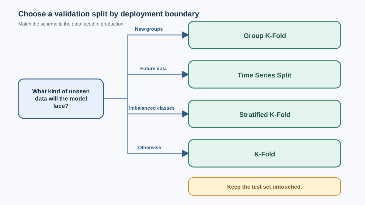
The splitter is a modeling decision, not a checkbox. Choosing the wrong one quietly inflates your reported accuracy, and you will not notice until the model underperforms in production.
Start with the deployment boundary, not with a default splitter. Ask what the model will face when it goes live, then work backward:
- Will the model predict on entirely new groups—new patients, new devices, new sessions? Enforce that boundary with group-aware folds.
- Will the model predict on future time periods? Enforce the time boundary with time-based splits.
- Is it classification with an imbalanced target? Add stratification to keep class proportions stable across folds.
- Otherwise? Plain k-fold is a solid default.
| Splitter | When to Use | What It Protects Against |
|---|---|---|
| K-Fold | General regression and well-balanced classification | Seed-dependent single splits |
| Stratified K-Fold | Classification, especially imbalanced targets | Folds missing the rare class |
| Repeated K-Fold | Small datasets, close model comparisons | Remaining split-to-split noise |
| Group K-Fold | Rows grouped by patient, session, device | Near-duplicate leakage across folds |
| Time Series Split | Temporal data | Models peeking at the future |
Whatever splitter you choose, one rule never changes: the final test set stays untouched until the very end. Cross-validation is a smarter way to spend your validation data. The test set remains the one honest measurement you get after all modeling decisions are final.
The Practical Takeaway
Ask one question before you run cross-validation: what must the validation fold not share with training? Same group, same time, same preprocessing. Answer that question honestly, choose the splitter that enforces the boundary, then run one clean cross-validation and read the mean and spread together.
The mean tells you the expected performance under your chosen validation design. The spread tells you how much to trust it. A model with a slightly lower mean and a much tighter spread is often the safer choice for real-world deployment—but check that the metric matches the cost of errors in your actual problem before treating that as a universal rule.
Once you have an honest cross-validation estimate, you have the tool you need for the next step: comparing models fairly and tuning hyperparameters without fooling yourself.
Knowledge check
Final check
Finish the article by checking the ideas you just learned.
References
Research updated Sep 8, 2026


