Compare Categorical Encodings in a Leakage-Safe Scikit-Learn Experiment

Swap OrdinalEncoder for OneHotEncoder, rerun the script, and the score moves. That single number feels like a verdict: one encoder is better. It isn't. You changed a representation, and the representation interacts with the model, the cardinality, and the split. The only way to learn what an encoder actually does is to change only the encoder and watch everything else hold still.

This tutorial builds that controlled comparison. You will run three encoders inside identical pipelines, inspect how each one reshapes the feature matrix, deliberately feed them a category they never saw during training, and read the held-out scores as evidence about one dataset rather than a universal ranking.

What Makes an Encoding Comparison Fair

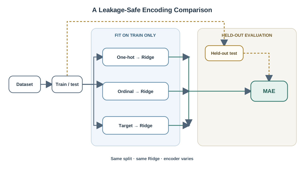
Before any code, fix the experimental contract. If you break it, the result is noise wearing a number.

Hold everything constant except the encoder. Same estimator, same train/test split, same random_state, same numeric preprocessing. The encoder is the only variable. If two things change, you cannot attribute the difference to either.

Fit every encoder inside a pipeline, on training data only. This is the leakage-safe preprocessing rule. If you fit an encoder on the full table and then split, the encoder has already seen the test categories. Its vocabulary is contaminated. The score goes up, and it means less.

You already know from working with pipelines that fit learns from data and transform applies what was learned. That separation is the whole point here: fit-time category knowledge stays attached to the training fold, and transform-time behavior stays consistent at prediction. An encoder fitted outside the pipeline breaks that contract silently.

State your success criteria now. Same folds across candidates, comparable feature counts you can explain, and a held-out score you can attribute to the encoder rather than to a changed split.

Set Up the Dataset and the Split

We need a table with at least one categorical column that has enough categories to make the comparison interesting, plus a numeric column. Here I'll use a small synthetic frame so the numbers are reproducible and the categories are visible. In your own work, load a real table with pandas.read_csv or pandas.read_parquet.

import numpy as np
import pandas as pd
from sklearn.model_selection import train_test_split

rng = np.random.default_rng(0)

# 'city' has 6 categories; 'rooms' is numeric.
cities = ["alpha", "bravo", "charlie", "delta", "echo", "foxtrot"]
n = 600
df = pd.DataFrame({
    "city": rng.choice(cities, size=n, p=[0.35, 0.25, 0.15, 0.1, 0.1, 0.05]),
    "rooms": rng.integers(1, 6, size=n),
})
# Target depends on city and rooms, plus noise.
city_effect = {"alpha": 0.0, "bravo": 1.0, "charlie": 2.0,
               "delta": 3.0, "echo": 4.0, "foxtrot": 5.0}
df["price"] = (df["city"].map(city_effect)
               + 0.8 * df["rooms"]
               + rng.normal(0, 0.5, size=n))

X = df[["city", "rooms"]]
y = df["price"]

X_train, X_test, y_train, y_test = train_test_split(
    X, y, test_size=0.25, random_state=42
)

Inspect the categorical column before you encode anything:

print(X_train["city"].value_counts())
print("distinct categories:", X_train["city"].nunique())

You should see six categories with uneven counts — foxtrot is rare. That rarity matters later. Environment assumptions: scikit-learn, pandas, and NumPy, with random_state=42 fixed so every number reproduces.

Build Three Candidate Pipelines

Each candidate wraps one encoder and the same estimator. I'll use Ridge so the linear model can weight each category independently — that makes the one-hot effect visible.

The critical detail is routing. Only city should pass through the encoder. rooms is already numeric and must stay untouched, or you are no longer comparing encoders — you are comparing encoders plus a changed numeric representation. A ColumnTransformer keeps that boundary explicit.

from sklearn.compose import ColumnTransformer
from sklearn.pipeline import Pipeline
from sklearn.preprocessing import OneHotEncoder, OrdinalEncoder, TargetEncoder
from sklearn.linear_model import Ridge

def make_pipeline(encoder):
    preprocess = ColumnTransformer(
        transformers=[("city", encoder, ["city"])],
        remainder="passthrough",   # 'rooms' passes through unchanged
    )
    return Pipeline([
        ("prep", preprocess),
        ("model", Ridge()),
    ])

candidates = {
    "onehot": make_pipeline(
        OneHotEncoder(handle_unknown="ignore")
    ),
    "ordinal": make_pipeline(
        OrdinalEncoder()
    ),
    "target": make_pipeline(
        TargetEncoder(cv=5, random_state=42)
    ),
}

Three encoders, one skeleton:

• One-hot produces one indicator column per training category. The model can assign each city its own weight.
• Ordinal produces a single integer column. It is cheap in dimensions, but it imposes an order the data may not have — alpha < bravo < charlie is a claim, not a fact.
• Target uses the label to build the representation. Because it reads y, it must be cross-fitted inside the pipeline; otherwise the label leaks into the features. The cv=5 argument handles that cross-fitting for you.

Inspect Feature Dimensions Before You Score

Representation size is a measurable property, not an abstraction. Fit each pipeline on the training data and print the transformed shape.

for name, pipe in candidates.items():
    pipe.fit(X_train, y_train)
    Xt = pipe.named_steps["prep"].transform(X_train)
    print(f"{name:8s} -> {Xt.shape}")

Expected output:

onehot   -> (450, 7)
ordinal  -> (450, 2)
target   -> (450, 2)

Read the arithmetic. One-hot adds roughly one column per observed category: six cities plus the untouched numeric rooms column gives seven. Ordinal and target each keep the original two columns. A column with many categories can multiply your feature matrix, and that growth is not free — more columns mean more split points for trees and more coefficients for linear models, which shows up as fit time and memory, not just accuracy.

Confirm which columns appeared instead of guessing:

print(candidates["onehot"].named_steps["prep"]
      .named_transformers_["city"].get_feature_names_out())

You should see city_alpha through city_foxtrot. The rooms column is still there, but it came through the passthrough branch, so it does not appear in the encoder's own feature names.

Test Unknown-Category Behavior on Purpose

The most common production failure is a category that appears only at prediction time. Turn it into a deliberate experiment. Build a small slice with a city that never appeared in training.

X_unseen = pd.DataFrame({"city": ["zulu"], "rooms": [3]})

for name, pipe in candidates.items():
    try:
        out = pipe.named_steps["prep"].transform(X_unseen)
        print(f"{name:8s} -> {out}")
    except Exception as e:
        print(f"{name:8s} -> ERROR: {type(e).__name__}")

What you'll observe:

• One-hot with handle_unknown="ignore" emits all zeros for that row — the model sees "none of the known cities."
• Ordinal raises an error by default. It has no integer to assign to zulu.
• Target falls back to a prior or global mean, because it has no target statistics for an unseen category.

This is a design decision, not a bug. The encoder's unknown-category policy defines what the model should assume when it meets something new, and you must choose it before deployment. Silently encoding unknowns as all-zeros is safe but discards information. Raising an error is loud but can halt a live prediction path. Neither is universally right.

Common mistake: Discovering your unknown-category policy in production, when a single unseen value crashes the prediction endpoint.

Score the Candidates and Read the Result Carefully

Evaluate each pipeline on the same held-out data with the same metric.

from sklearn.metrics import mean_absolute_error

for name, pipe in candidates.items():
    preds = pipe.predict(X_test)
    print(f"{name:8s} MAE = {mean_absolute_error(y_test, preds):.3f}")

On this synthetic data, one-hot and target tend to land close together, with ordinal trailing — because ordinal forces an arbitrary numeric order onto cities that have no natural order, and the linear model can only scale that single column. But read the pattern, not the ranking. A linear model usually benefits from one-hot because it can weight each category independently. Tree models often tolerate ordinal or native categorical handling, because they can split the integer column into ranges.

State the boundary out loud: this is one dataset, one split, one seed, one estimator. A different table can reverse the ordering. If the scores are close, treat the cheaper representation as the reasonable default rather than chasing noise.

Failure Modes and Debugging Signals

The symptoms below tell you the experiment is broken, not just the model.

• A suspiciously high score is the first sign of leakage. Check whether any encoder was fitted before the split.
• A shape mismatch at predict time usually means the encoder was fitted on a different set of categories than the one being transformed.
• A silent all-zeros row is the fingerprint of handle_unknown="ignore" meeting an unseen category. It is correct behavior, but it should be a conscious choice.
• A target encoder that scores beautifully in-sample and poorly out-of-sample is the classic sign that cross-fitting was skipped.

One Modification Worth Running Next

Change one variable at a time. Swap Ridge for a tree-based model and rerun the same three pipelines. Or collapse rare categories with min_frequency and watch the feature count and unknown-category behavior change together. Or add a second categorical column with much higher cardinality and watch the one-hot dimension count grow.

Before you run it, predict the outcome. A prediction that fails teaches more than a result that merely confirms.

Where This Leaves You

Pick the encoder that fits your model and your cardinality, verify unknown-category behavior deliberately, and keep the whole thing inside a training-fitted pipeline. The score is evidence about one dataset, not a verdict on encoders in general. The next natural step is running this same controlled comparison across different estimators, or adding a higher-cardinality column to see where the representation cost starts to bite.