Fit a Leakage-Safe Scikit-Learn Pipeline on Tabular Data

You scale the whole table, split it, train a model, and get 0.94. You ship it, and real data hands you 0.71. Nothing broke in production. The break happened earlier, when a mean computed from your test rows quietly walked into training.

Here is the fix, built one step at a time: a single pipeline object that learns only from training rows, plus a validation check that leaves your final test set sealed.

The Setup: One Table, Three Sealed Boxes

We need a small table with mixed column types and a few missing values, so preprocessing has real work to do. I will build one inline so you can run this end to end without downloading anything.

import numpy as np
import pandas as pd
from sklearn.model_selection import train_test_split

rng = np.random.default_rng(0)
n = 400

df = pd.DataFrame({
    "age": rng.integers(18, 70, n).astype(float),
    "income": rng.normal(52000, 15000, n).round(0),
    "plan": rng.choice(["basic", "plus", "pro"], n),
    "region": rng.choice(["north", "south", "east", "west"], n),
    "churned": rng.integers(0, 2, n),
})

# Punch holes so imputation has something to learn.
df.loc[rng.choice(n, 40, replace=False), "age"] = np.nan
df.loc[rng.choice(n, 25, replace=False), "income"] = np.nan
df.loc[rng.choice(n, 30, replace=False), "plan"] = np.nan

X = df.drop(columns="churned")
y = df["churned"]

Dependencies are just pandas, NumPy, and scikit-learn. No services, no credentials. Every random operation uses a fixed seed so your numbers match mine.

Now the split discipline. Two splits, in order:

X_pool, X_test, y_pool, y_test = train_test_split(
    X, y, test_size=0.2, stratify=y, random_state=42
)
X_train, X_val, y_train, y_val = train_test_split(
    X_pool, y_pool, test_size=0.25, stratify=y_pool, random_state=42
)

print(X_train.shape, X_val.shape, X_test.shape)
print(y_train.mean().round(3), y_val.mean().round(3), y_test.mean().round(3))

Expected shapes: (240, 4) (80, 4) (80, 4). The three churn rates should land near each other because stratify preserves the class ratio in every split.

The test set is now sealed. It does not appear again in this article. If you are fuzzy on why, the short version: fit learns, transform applies, and only training rows are allowed to teach. The working pool gets split into train and validation so you have an honest check that is not the final exam.

Build the Preprocessing Steps

Before bundling anything, build the transformations as standalone objects. You want to see what each one learns.

from sklearn.impute import SimpleImputer
from sklearn.preprocessing import StandardScaler, OneHotEncoder
from sklearn.compose import ColumnTransformer

numeric_cols = ["age", "income"]
categorical_cols = ["plan", "region"]

numeric_pipe = [
    ("impute", SimpleImputer(strategy="median")),
    ("scale", StandardScaler()),
]

categorical_pipe = [
    ("impute", SimpleImputer(strategy="most_frequent")),
    ("encode", OneHotEncoder(handle_unknown="ignore")),
]

preprocessor = ColumnTransformer([
    ("num", numeric_pipe, numeric_cols),
    ("cat", categorical_pipe, categorical_cols),
])

Read that carefully, because every step hides a learned quantity. The median imputer stores a median. The scaler stores a mean and a standard deviation. The encoder stores a category vocabulary. None of those are constants you typed. All of them are estimates pulled from data, which means all of them can leak.

ColumnTransformer routes each column group to the right path and keeps the output aligned, so age never gets one-hot encoded and plan never gets scaled.

Common mistake: a misspelled column name in numeric_cols or categorical_cols does not raise an error by default. The column is silently dropped, and your model trains on less information than you think. Print the structure and check the column count before you trust it.

To inspect what the preprocessor learns, fit a throwaway copy on the training rows. Keep the original object untouched so the pipeline can fit it cleanly later:

from sklearn.base import clone

inspection_copy = clone(preprocessor).fit(X_train)
print(inspection_copy.get_feature_names_out())

You should see num__age, num__income, and one cat__plan_* / cat__region_* entry per observed category. If a column you expected is missing, fix the name list now.

Wrap Preprocessing and Model in One Pipeline

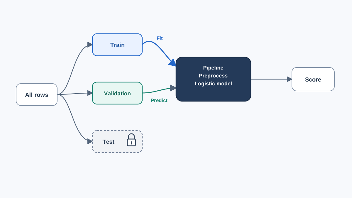
Now combine the preprocessor and an estimator into a single object. This is the step that turns leakage safety from a habit into a structural property.

from sklearn.pipeline import Pipeline
from sklearn.linear_model import LogisticRegression

clf = Pipeline([
    ("prep", preprocessor),
    ("model", LogisticRegression(max_iter=1000)),
])

clf.fit(X_train, y_train)
print(clf.score(X_train, y_train).round(3))

When you call fit, the pipeline walks its steps in order. The preprocessor fits on training rows, transforms them, and hands the result to the logistic regression, which fits on that transformed matrix. Nothing outside X_train was consulted. The preprocessor object you built earlier is fitted here, inside the pipeline's own fit call — not before it.

Contrast that with the manual version: fit the scaler on the full table, then split, then train. The scaler's mean now contains information from rows that will later be used to judge the model. That is the leak. It is small, it is invisible in your score, and it is still a broken boundary.

The named steps matter for a second reason. You can reach into any parameter with double underscores:

clf.set_params(model__C=0.5)

That syntax is what makes tuning possible later, because a search procedure needs an addressable path to every knob.

One warning about the number you just printed: the training score is not evidence of generalization. A model can memorize its training rows and score near 1.0 while being useless on anything new. That is exactly why the next section exists.

Check Predictions on the Validation Portion

Call predict on the validation features:

from sklearn.metrics import accuracy_score

val_pred = clf.predict(X_val)
print(accuracy_score(y_val, val_pred).round(3))

The pipeline applies the transformations it already fitted. It does not re-learn anything from validation rows. That is the whole point of transform versus fit_transform, and the pipeline handles the distinction for you.

Now compare the two numbers. A large gap between training and validation accuracy is an overfitting signal. A suspiciously tiny gap on a small dataset usually means the split is too easy or too small to be informative, not that you have solved machine learning.

Aggregate numbers hide specific failures, so look at a few rows directly:

check = pd.DataFrame({
    "actual": y_val.values[:10],
    "predicted": val_pred[:10],
})
print(check)

If the predictions look inverted or systematically shifted, you likely have a label-encoding mistake that a single accuracy figure would happily average away.

Validation rows may inform your choices. The test set has still seen nothing.

Note: one validation split on a few hundred rows is a noisy estimate. Treat the number as a rough reading, not a verdict. The size of any leakage effect also depends heavily on dataset size and the type of leakage involved, so do not expect a dramatic gap here.

Break It on Purpose: A Leakage Experiment

Do not take the rule on faith. Build the wrong version and watch what happens.

leaky_scaler = StandardScaler().fit(X_pool[["age", "income"]])
leaky_encoder = OneHotEncoder(handle_unknown="ignore").fit(
    X_pool[["plan", "region"]]
)

def leaky_features(frame):
    num = leaky_scaler.transform(frame[["age", "income"]])
    cat = leaky_encoder.transform(frame[["plan", "region"]])
    return np.hstack([num, cat.toarray()])

leaky_model = LogisticRegression(max_iter=1000).fit(
    leaky_features(X_train), y_train
)
leaky_val_score = accuracy_score(
    y_val, leaky_model.predict(leaky_features(X_val))
)
print(leaky_val_score.round(3))

Those two transformer objects learned from all 320 working rows, including the 80 that serve as validation. The model then trains and scores on features built from that contaminated state. Compare leaky_val_score against the leakage-safe pipeline's validation score.

On a dataset this small, the two numbers may be nearly identical. That is the lesson, not a contradiction. The problem is not the size of the distortion. The problem is that information crossed a boundary it was never allowed to cross, and you can no longer trust the number as an estimate of future performance.

Preprocessing leakage is also one class among several. Selection leakage, where you peek at validation results while choosing features or hyperparameters, tends to produce much larger distortions at practical dataset sizes. The mechanism is the same in every case: something learned from evaluation data influenced training.

So here is the decision rule I use: any learned preprocessing or feature-selection step used during evaluation belongs inside the pipeline. That placement is what forces the correct fit boundary — training rows only, refit inside every cross-validation fold. It is not a blanket ban on ever calling fit outside a pipeline; it is a rule about which data is allowed to teach the object that produces your evaluation features.

One Modification to Try Next

Add a feature-selection step inside the pipeline and watch it obey the same rule:

from sklearn.feature_selection import SelectKBest, f_classif

clf2 = Pipeline([
    ("prep", preprocessor),
    ("select", SelectKBest(f_classif, k=4)),
    ("model", LogisticRegression(max_iter=1000)),
])
clf2.fit(X_train, y_train)
print(accuracy_score(y_val, clf2.predict(X_val)).round(3))

The selector computes F-scores against the target. If you fit it outside the pipeline on all working rows, those scores were influenced by validation labels. Inside the pipeline, it only sees training rows.

I chose k=4 deliberately. The encoded feature count depends on which categories appear in the training split, and with three plan values and four region values you are guaranteed at least four encoded columns even if a category is missing. Picking k=6 would risk a runtime error on an unlucky split, which would distract you from the actual lesson. If you want a larger k, derive it from the fitted preprocessor's output width instead of guessing.

Before you run it, predict the direction of the change. Then run it and compare.

Alternatively, swap the estimator for a tree-based model. Scaling becomes unnecessary because trees split on thresholds rather than distances, but encoding still matters because trees cannot consume raw strings. That is a concrete reminder that preprocessing choices depend on the model, not on habit.

Where This Leaves You

Keep the fitted pipeline object. It is not a one-off script. It is the same object you hand to cross-validation or a hyperparameter search later, and because preprocessing lives inside it, every fold refits its own transformations on its own training rows. That is why building it correctly now pays off immediately.

The durable rule is short enough to remember: anything that learns from data lives inside the pipeline, and the test set stays sealed until the very end. Your next move is to take this exact pipeline and run it through cross_val_score, then compare the fold scores against the single validation number you just computed.