Compare Scikit-Learn Pipeline Models Without Touching the Test Set

You have three pipelines. Their scores are close enough that the ranking feels like a coin flip. So you run them against the test set to break the tie — and in that moment, the test set stops being a test set.

Here is the rule that fixes this: all comparison happens inside the training data. The test set is opened once, at the end, for the pipeline you already chose.

This article assumes you can already split data, build a leakage-safe pipeline, and recognize cross-validation when you see it. If any of those feel shaky, the earlier pieces in this category cover them. What we are doing here is turning those tools into a comparison procedure you can trust.

Why Comparing on the Test Set Breaks the Comparison

The test set has exactly one job: to give you a final, unbiased estimate of how your chosen model will behave on data it has never seen. It is a measurement instrument, not a tuning dial.

Every time you pick a winner by test score, you leak selection information into the test set. You are no longer asking "how well does this model generalize?" You are asking "which of these models happens to fit this particular sample best?" Those are different questions, and only the first one is useful.

The failure mode is quiet. A beginner tries five pipelines against the test set, reports the best one, and feels good about the number. What actually happened is that the test set became a validation set, and the reported score is now optimistic. The model was selected because it scored well on that specific data.

Common mistake: Treating the test set as a tiebreaker. A tiebreaker is a decision signal, and decision signals belong in training.

The practical rule is short: comparison and selection happen on training data only. The test set is opened exactly once, for the pipeline you have already committed to.

Set Up the Comparison: One Split, Many Candidates

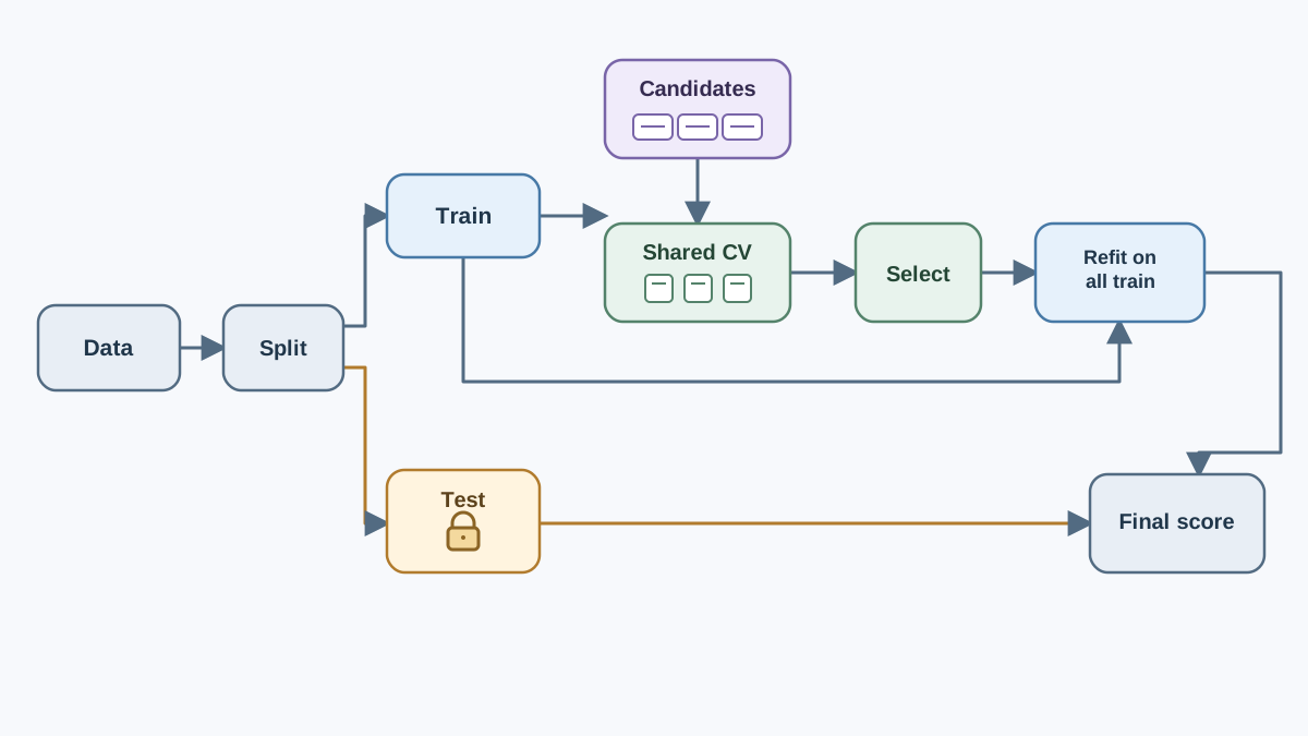
Start with the smallest runnable setup. You need Python with scikit-learn, NumPy, and pandas. We will use the breast cancer dataset that ships with scikit-learn, so the example runs without any downloads. It has 30 numeric features and a binary target — no categorical columns to encode, which keeps the comparison focused on the pipelines themselves.

import numpy as np
import pandas as pd
from sklearn.datasets import load_breast_cancer
from sklearn.model_selection import train_test_split

data = load_breast_cancer()
X = pd.DataFrame(data.data, columns=data.feature_names)
y = data.target

X_train, X_test, y_train, y_test = train_test_split(
    X, y, test_size=0.2, random_state=42, stratify=y
)

print("Training rows:", len(X_train))
print("Test rows:", len(X_test))
print("Test set is now sealed. Do not reference X_test or y_test again.")

Two things to notice. First, random_state=42 makes the split reproducible — same rows every run. Second, stratify=y keeps the class proportions similar in both halves, which matters for classification. If you are doing regression, drop the stratify argument.

Now define your candidates. Each candidate must be a full pipeline, not a bare estimator. That means the preprocessing travels with the model, so no transformation is ever fit outside the comparison.

from sklearn.pipeline import Pipeline
from sklearn.preprocessing import StandardScaler, MinMaxScaler
from sklearn.linear_model import LogisticRegression
from sklearn.ensemble import RandomForestClassifier

candidates = {
    "logreg_standard": Pipeline([
        ("scaler", StandardScaler()),
        ("clf", LogisticRegression(max_iter=1000)),
    ]),
    "logreg_minmax": Pipeline([
        ("scaler", MinMaxScaler()),
        ("clf", LogisticRegression(max_iter=1000)),
    ]),
    "forest": Pipeline([
        ("clf", RandomForestClassifier(random_state=42)),
    ]),
}

for name in candidates:
    print(name)

This candidate set isolates a real choice: does the scaler matter for logistic regression, and does a tree-based model beat both? You are not comparing random things. You are comparing hypotheses.

Note: If your own data has categorical columns, every candidate pipeline needs a ColumnTransformer that encodes them before the estimator sees them. A StandardScaler cannot process strings, and a random forest cannot either. The comparison logic below is identical — only the preprocessing step changes.

Score Every Candidate With the Same Cross-Validation

Here is the comparison loop. It runs entirely on the training data.

from sklearn.model_selection import StratifiedKFold, cross_val_score

cv = StratifiedKFold(n_splits=5, shuffle=True, random_state=42)

for name, pipe in candidates.items():
    scores = cross_val_score(pipe, X_train, y_train, cv=cv, scoring="accuracy")
    print(f"{name}: mean={scores.mean():.3f} std={scores.std():.3f}")
    print(f"  folds: {np.round(scores, 3)}")

Expected output looks roughly like this:

logreg_standard: mean=0.974 std=0.011
  folds: [0.97 0.98 0.96 0.97 0.99]
logreg_minmax: mean=0.971 std=0.013
  folds: [0.96 0.98 0.96 0.97 0.98]
forest: mean=0.958 std=0.015
  folds: [0.95 0.97 0.94 0.96 0.97]

The numbers will differ on your data, but the structure is what matters. Three details make this comparison fair:

The same cv object is reused for every candidate. If candidate A is scored on different folds than candidate B, the difference you see might be fold luck, not model quality. Same folds, same random state, same metric.

Each pipeline is passed directly to cross_val_score. Scikit-learn clones the pipeline and refits every step inside each fold. The scaler learns its mean and standard deviation from the fold's training portion only. That is the whole point of wrapping preprocessing in a pipeline.

The metric is chosen before you look at results. Pick it from the cost of mistakes — false positives versus false negatives — not from whichever number happens to look best afterward.

Read the Results Without Fooling Yourself

Compare means alongside their spread. A 0.01 gap in means sitting inside a 0.02 standard deviation is not a verdict. It is noise wearing a ranking costume.

Look at the example above. logreg_standard leads at 0.974, but its standard deviation is 0.011, and forest sits at 0.958 with a standard deviation of 0.015. The gap between the top two is real enough to notice, but the gap between the two logistic regression variants is not — 0.974 versus 0.971 is well inside the fold-to-fold wobble.

When the dataset is small or classes are imbalanced, use StratifiedKFold (as above) or repeated cross-validation to get a more stable estimate. More folds and more repeats cost compute, but they shrink the noise you are trying to see through.

Watch for one tell-tale sign of a broken comparison: a candidate that scores suspiciously high. That usually means a transformation was fit outside the pipeline — on the full training set, or worse, on everything. The scaler saw data it should not have seen, and the score inflated accordingly.

Tip: When scores are within noise, prefer the simpler pipeline. Complexity has to earn its place with a visible, repeatable gain — not a lucky fold.

One honest limit: cross-validation estimates performance on data resembling the training distribution. It cannot rescue a bad split, a leaked feature, or a target that encodes the answer.

Select a Pipeline and Tune It Inside the Training Data

Pick the winner on validation evidence, and write down why — the criterion, not just the name. "Logistic regression with standard scaling won on mean accuracy with the tightest spread" is a decision. "Logistic regression looked best" is a guess.

If you want to tune hyperparameters, the search itself is part of selection, so it stays inside the training data:

from sklearn.model_selection import GridSearchCV

param_grid = {
    "clf__C": [0.01, 0.1, 1.0, 10.0],
}

search = GridSearchCV(
    candidates["logreg_standard"], param_grid, cv=cv, scoring="accuracy"
)
search.fit(X_train, y_train)

print("Best params:", search.best_params_)
print("Best CV score:", round(search.best_score_, 3))

Notice the double underscore in clf__C. That is how you address a parameter inside a pipeline step: stepname__parametername.

Common mistake: Running a grid search on the full dataset and reporting the best score as a generalization estimate. The search tried many configurations and kept the one that fit best. That is selection, and selection needs its own validation.

If you want an unbiased estimate of the entire selection-and-tuning procedure — not just the final model — nested cross-validation is the honest option. The inner loop tunes, the outer loop evaluates. It costs more compute, and for many beginner projects the simpler approach is enough. But know that it exists, and know when you need it.

Open the Test Set Once

This is the moment. Fit the selected pipeline on the full training data, then score it on the test set exactly once.

final_pipeline = search.best_estimator_
final_pipeline.fit(X_train, y_train)

test_score = final_pipeline.score(X_test, y_test)
print(f"Final test score: {test_score:.3f}")

Compare that number to the cross-validated estimate. If cross-validation said 0.974 and the test set says 0.965, you are in good shape — the estimate held. If the test score drops sharply, that is a signal to investigate, not a reason to re-tune against the test set.

What does the test score actually mean? It is one sample of an estimate, not a guarantee. A small test set makes it noisier. A test set drawn from a different time period or population than training makes it misleading.

If the test score disappoints, the honest move is to return to the training data, revise your hypothesis, and accept that this test set is now spent for this round. You can split off a new one if you have more data. You cannot un-see the old one.

Record the number and the pipeline configuration that produced it. Reproducibility means the next person — including future you — can rerun the experiment and get the same result.

A Small Experiment: Change One Thing

Reading about leakage is not the same as feeling it. Let's break the boundary on purpose.

from sklearn.preprocessing import StandardScaler
from sklearn.linear_model import LogisticRegression
from sklearn.model_selection import cross_val_score

# Deliberately wrong: fit the scaler on ALL training data first
scaler = StandardScaler()
X_train_scaled = scaler.fit_transform(X_train)

leaky_scores = cross_val_score(
    LogisticRegression(max_iter=1000), X_train_scaled, y_train, cv=cv
)
print(f"Leaky: mean={leaky_scores.mean():.3f} std={leaky_scores.std():.3f}")

Run this, then run the correct pipeline version from earlier. The success criterion is not a specific score movement — it is that you can point to where the scaler was fit. In the leaky version, fit_transform ran once on the entire training set before any fold was created. Every fold's validation rows contributed their mean and spread to the scaler that then transformed them. In the pipeline version, the scaler refits inside each fold, so validation rows never touch the statistics used to transform them.

The score difference may be large, small, or even reversed on a particular dataset. That is the point: you cannot diagnose leakage by watching the score direction. You diagnose it by tracing the fit boundary. If any transformation learned from rows that later appear in a validation fold, the comparison is compromised regardless of what the number says.

Try one more variation. Swap StandardScaler for MinMaxScaler, or add a feature-selection step, and rerun the same cross-validation. Does the ranking change? By how much? Building intuition for "how big a gap is real" is the skill that separates a comparison from a coin flip.

The Rule You Keep

Compare inside the training data. Choose on validation evidence. Spend the test set once.

That is the whole workflow, and it scales from three pipelines to thirty. The mechanism does not change: every decision that shapes the model must be made without the test set watching.

Your next step is error analysis. You have a chosen pipeline and one honest test score — now ask where it fails. Which rows does it get wrong? Are the mistakes clustered in a particular class, a particular region of the feature space, a particular time period? That question moves you from "how good is this model?" to "what is this model actually learning?" — and it is where real improvement usually starts.