Compare Imputation Strategies in a Leakage-Safe Scikit-Learn Pipeline

Fill the missing values, split the data, train the model, and watch your score climb. It feels like progress. It is usually a leak.

Here is the trap. You have a table with holes in it. You replace every hole with the column mean, then split into train and test, then train a model. The test score looks great. But the mean you used to fill those holes was computed from every row — including the rows you later called "test." The held-out data already whispered its secrets into your training features. You cannot tell whether the imputation helped or the leak did.

This tutorial builds a controlled experiment instead. We change exactly one thing between runs — the imputation strategy — and hold the dataset, the split, the estimator, and the metric fixed. Four pipelines. One honest comparison.

Why a Fair Imputation Comparison Is Harder Than It Looks

A single RMSE number is not evidence. It is a result under specific conditions. Change the conditions and the number changes. So if you want to know whether mean or median imputation is better for your data, you have to freeze everything else.

The most common beginner move is to impute the whole dataframe first, then split. That order lets held-out rows influence the fill values. The fix is simple to state and easy to get wrong: split first, then fit every learned transformation on training rows only.

This is the same boundary you already met when learning about pipelines and train/test splits. A pipeline keeps fit (learning) and transform (applying) separate, so the imputer learns its fill values from training data and applies them everywhere else. We lean on that here rather than re-explaining it.

Our protocol:

• Same dataset, same random seed.
• Same holdout, reserved before any preprocessing.
• Same estimator, same metric.
• Only the imputer configuration changes.

Set Up the Experiment: Dataset, Holdout, and Injected Missingness

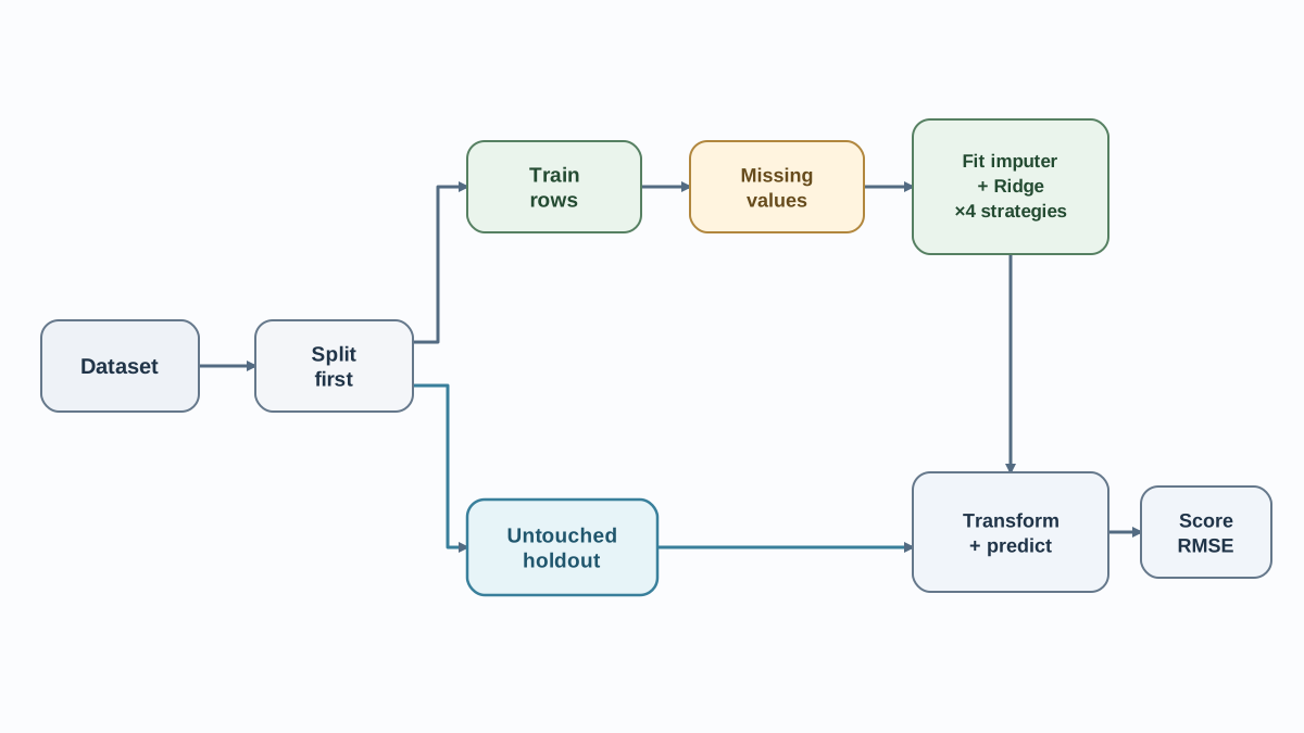
We need a numeric regression problem with known ground truth, so we can inject missing values on purpose and document exactly how many we removed.

import numpy as np
from sklearn.datasets import make_regression
from sklearn.model_selection import train_test_split

RANDOM_STATE = 42
MISSING_FRACTION = 0.20

X, y = make_regression(
    n_samples=1000, n_features=8, n_informative=6,
    noise=10.0, random_state=RANDOM_STATE,
)

X_train, X_holdout, y_train, y_holdout = train_test_split(
    X, y, test_size=0.2, random_state=RANDOM_STATE,
)

The holdout is now locked. We will not touch it again until we score the four pipelines.

Next, inject missing values into the training features only. The holdout stays complete, which keeps the final score comparable across runs.

rng = np.random.default_rng(RANDOM_STATE)
mask = rng.random(X_train.shape) < MISSING_FRACTION
X_train_missing = X_train.copy()
X_train_missing[mask] = np.nan

missing_per_column = np.isnan(X_train_missing).sum(axis=0)
print("Missing per column:", missing_per_column)
print("Total missing:", missing_per_column.sum())

Because the generator is seeded, this experiment is repeatable. Run it tomorrow and you get the same holes in the same places. That reproducibility is the whole point — a comparison you cannot re-run is not a comparison.

Build the Four Pipelines

Here is the smallest useful pipeline. The imputer lives inside it, so it can only ever see the rows passed to fit.

from sklearn.pipeline import Pipeline
from sklearn.impute import SimpleImputer
from sklearn.linear_model import Ridge

def make_pipeline(strategy, add_indicator):
    return Pipeline([
        ("imputer", SimpleImputer(
            strategy=strategy, add_indicator=add_indicator)),
        ("model", Ridge()),
    ])

Why does the imputer have to be inside the pipeline? Because a pipeline is a single object with one fit method. When you call pipe.fit(X_train_missing, y_train), scikit-learn fits the imputer on the training rows, transforms them, and hands the result to the model. At predict time it applies the same learned fill values to new rows. If you fit the imputer separately first, you have to remember to transform the holdout with training statistics — and the moment you forget, or the moment you add cross-validation, the boundary breaks.

The four configurations differ only in two arguments:

Run	strategy	add_indicator
1	"mean"	False
2	"median"	False
3	"mean"	True
4	"median"	True

Everything else — the estimator, the split, the random state — is byte-for-byte identical.

What the Missingness Indicator Actually Adds

Before we run anything, understand what add_indicator=True does. It appends one binary column per feature that contained at least one missing value. A row gets a 1 in that column if its original value was missing, and a 0 otherwise.

Why would that help? Because sometimes the fact that a value is missing carries signal. If a sensor drops out only when it overheats, the absence is information. The indicator lets the model learn a separate effect for "this was missing" instead of only seeing the imputed substitute, which is a guess.

Two things to verify explicitly:

• The indicator feature count should equal the number of features that had at least one missing value — not the total feature count.
• If a column had no missing values, it gets no indicator column.

Common mistake: Assuming you always get one indicator per feature. You get one per feature that actually had missingness in the training data. On a different split, that count can change.

When indicators help: missingness is not random and correlates with the target. When they hurt: they add near-constant columns that mostly encode noise, which can encourage overfitting on small datasets.

Run the Comparison and Read the Results

Now fit each pipeline on training rows, predict on the untouched holdout, and score with one metric function.

from sklearn.metrics import root_mean_squared_error

configs = [
    ("mean", False),
    ("median", False),
    ("mean", True),
    ("median", True),
]

for strategy, add_indicator in configs:
    pipe = make_pipeline(strategy, add_indicator)
    pipe.fit(X_train_missing, y_train)
    preds = pipe.predict(X_holdout)
    rmse = root_mean_squared_error(y_holdout, preds)
    n_features_out = pipe.named_steps["imputer"].transform(
        X_train_missing).shape[1]
    print(f"{strategy:>6} | indicator={add_indicator!s:<5} "
          f"| RMSE={rmse:7.3f} | features out={n_features_out}")

You should see four RMSE values and, for the indicator runs, a feature count larger than eight. The exact numbers depend on your seed and data — that is expected. What matters is that all four ran, none crashed, and no imputer ever saw a holdout row.

Read the results with discipline:

• A small gap between mean and median is normal. On roughly symmetric data, the two fill values land close together, so the model barely notices the difference.
• A lower RMSE here does not crown a winner. It means that on this dataset, with this seed and this estimator, one configuration scored better. Change the data and the ranking can flip.
• The indicator variants may or may not pull ahead. If missingness is random noise, they add columns without adding signal.

Note: The value of this experiment is the protocol, not the winning row. You now have a way to ask the question honestly.

Debug the Three Failures Beginners Hit

Remaining NaNs after transform. If transform still returns NaNs, you likely have a column that was entirely missing in the training data — SimpleImputer drops all-missing columns by default — or a dtype it cannot fill. Check missing_per_column and look for a column equal to the row count.

Indicator-column mismatch. The indicator count reflects only columns with observed missingness. If you expected eight extra columns and got six, two features had no missing values in training. That is correct behavior, not a bug.

Preprocessing fitted outside the pipeline. The fingerprint is a score that shifts when you reorder or resplit the data. If your RMSE changes just because you shuffled rows, a learned statistic leaked across the boundary. Move the imputer back inside the pipeline.

Change the Missing Fraction and Re-run

The real payoff is turning this into a reusable script. Change one number and run it again:

MISSING_FRACTION = 0.40

Re-inject, rebuild the same four pipelines, and compare. A plausible pattern is that the indicator variants gain ground as missingness grows, because the model has more reason to distinguish "missing" from "imputed." Treat that as a hypothesis to test on your data, not a rule.

Notice the boundary of this experiment: we compared simple univariate strategies only. Model-based approaches like IterativeImputer or KNNImputer are a different question for a different article.

Where to Go Next

The lesson is not "median beats mean." The lesson is that you cannot pick an imputation strategy from a single score, and you must never let the holdout influence the fill values.

Keep this comparison as a script. Swap in a different estimator, or a different missing fraction, and watch whether the ranking holds. When it does not, you have learned something real about your data — and that is worth more than any one number.