Test SVM Scaling, Kernels, and Regularization With Scikit-Learn

Same data. Same SVC call. One run scores 0.85, the next 0.55, and the only thing that changed was whether you scaled the features first.

That gap is not noise. It is the SVM telling you what it actually cares about: distance. This article is a controlled experiment, not a hunt for a "best" model. You will change one knob at a time and watch the decision boundary move. By the end you will have a leakage-safe workflow you can rerun on your own data, plus the judgment to read a boundary plot instead of trusting a single accuracy number.

If you have not yet met margins, support vectors, and kernels, read the conceptual SVM material first. Here we assume you know what a train/test split is and want to see the mechanics in code.

Why the Same SVC Gives Different Answers

An SVM separates classes by margin geometry. It measures distances between points and the boundary, so the units of each feature directly shape that boundary. A feature measured in thousands and a feature measured in decimals do not contribute equally to a distance calculation unless you put them on comparable footing.

make_moons has two features on comparable ranges, which makes it a clean teaching case. It is also a slightly misleading one: because the ranges already match, you might conclude scaling never matters. It does. On real tabular data, feature ranges diverge wildly, and the unscaled model quietly degrades.

Here is the contract for everything that follows:

• One fixed stratified split, one seed.
• One knob changed at a time.
• Every comparison uses the same held-out data.

Along the way we will debug three failure modes: preprocessing before the split, mismatched feature dimensions when plotting, and runaway C or gamma.

Set Up the Dataset and the Fixed Split

import numpy as np
from sklearn.datasets import make_moons
from sklearn.model_selection import train_test_split

X, y = make_moons(n_samples=400, noise=0.25, random_state=42)
X_train, X_test, y_train, y_test = train_test_split(
    X, y, test_size=0.3, stratify=y, random_state=42
)

print(X_train.shape, X_test.shape)
print(np.bincount(y_train), np.bincount(y_test))

The noise=0.25 matters. Without noise, the two moons are trivially separable and every kernel looks brilliant. Noise forces the model to make real tradeoffs.

stratify=y keeps the class proportions consistent across both splits, so a lucky or unlucky split does not distort your comparison. The random_state freezes the split. Change it later and every number in this article becomes a different experiment.

Build the Pipeline Before You Touch the Model

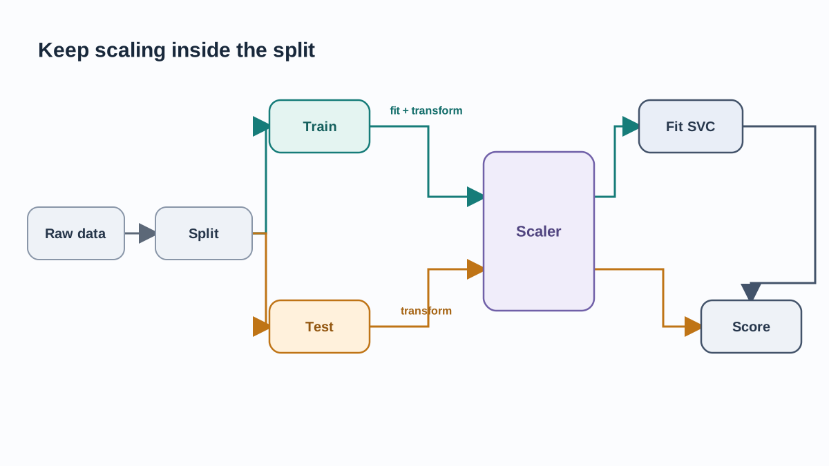
The smallest useful implementation wraps the scaler and the classifier together:

from sklearn.pipeline import make_pipeline
from sklearn.preprocessing import StandardScaler
from sklearn.svm import SVC

pipe = make_pipeline(StandardScaler(), SVC(kernel="rbf", C=1.0))
pipe.fit(X_train, y_train)
print(pipe.score(X_test, y_test))

That single line is doing something important. Inside a pipeline, StandardScaler is fit only on the training data, then applied to the test data using the training mean and variance. The test set never influences the scaling statistics.

The tempting shortcut breaks this:

# Do not do this
scaler = StandardScaler()
X_scaled = scaler.fit_transform(X)          # leaks test statistics
X_train, X_test, y_train, y_test = train_test_split(X_scaled, y, random_state=42)

Here the scaler saw the entire dataset before the split. The test set's mean and variance leaked into the transformation, and your held-out score is no longer honest. The pipeline form makes the correct behavior the default rather than a thing you remember to do.

If you want to inspect or swap steps, the explicit form is equivalent:

from sklearn.pipeline import Pipeline

pipe = Pipeline([
    ("scaler", StandardScaler()),
    ("svc", SVC(kernel="rbf", C=1.0)),
])
print(pipe.named_steps["svc"])

Scaled vs Unscaled: One Estimator, Two Boundaries

Now isolate scaling. Fit the same configuration twice — once bare, once wrapped.

bare = SVC(kernel="rbf", C=1.0).fit(X_train, y_train)
scaled = make_pipeline(StandardScaler(), SVC(kernel="rbf", C=1.0)).fit(X_train, y_train)

print("bare  :", bare.score(X_test, y_test))
print("scaled:", scaled.score(X_test, y_test))

On make_moons the unscaled boundary is usually visibly worse, because the RBF kernel's distance calculation is dominated by whichever feature happens to have the larger spread. Scaling changes the geometry the kernel sees, and that geometry is the whole model.

Two cautions. First, a single split is one sample of evidence. A large gap is informative; a small gap is not proof that scaling is irrelevant. Second, do not read this as "scaling always wins." Read it as: the kernel operates on distances, so you must control the units those distances are measured in.

Vary Kernel and C in a Small Controlled Grid

Keep the grid deliberately small so every cell is interpretable. We hold gamma at its default here on purpose, so the next section can isolate it.

import pandas as pd

rows = []
for kernel in ["linear", "rbf"]:
    for C in [0.1, 1.0, 100.0]:
        model = make_pipeline(StandardScaler(), SVC(kernel=kernel, C=C))
        model.fit(X_train, y_train)
        rows.append({
            "kernel": kernel,
            "C": C,
            "train": round(model.score(X_train, y_train), 3),
            "test": round(model.score(X_test, y_test), 3),
        })

print(pd.DataFrame(rows).to_string(index=False))

C trades off margin violations against simplicity. Low C tolerates violations for a smoother boundary; high C pushes toward classifying every training point correctly. The table exposes the pattern:

kernel	C	train	test
linear	0.1	0.821	0.817
linear	1.0	0.836	0.825
linear	100.0	0.836	0.825
rbf	0.1	0.850	0.842
rbf	1.0	0.968	0.942
rbf	100.0	0.996	0.933

Read the shape, not the exact digits. The linear kernel plateaus: raising C from 1 to 100 changes nothing, because a straight cut simply cannot bend around the moons. The RBF kernel at C=1.0 reaches the best test score here, while C=100.0 pushes training accuracy to near-perfect and lets test accuracy slip — the classic signature of a model memorizing the noise. Where train and test scores diverge, the model is fitting the split, not the pattern.

Read the Decision Boundaries, Not Just the Scores

Scores hide the shape of the decision. Plot it.

import matplotlib.pyplot as plt

def plot_boundary(model, X, y, ax, title):
    x_min, x_max = X[:, 0].min() - 0.5, X[:, 0].max() + 0.5
    y_min, y_max = X[:, 1].min() - 0.5, X[:, 1].max() + 0.5
    xx, yy = np.meshgrid(
        np.linspace(x_min, x_max, 300),
        np.linspace(y_min, y_max, 300),
    )
    grid = np.c_[xx.ravel(), yy.ravel()]
    Z = model.predict(grid).reshape(xx.shape)
    ax.contourf(xx, yy, Z, alpha=0.3, cmap="coolwarm")
    ax.scatter(X[:, 0], X[:, 1], c=y, edgecolor="k", s=20)
    ax.set_title(title)

models = [
    ("linear, C=1", make_pipeline(StandardScaler(), SVC(kernel="linear", C=1.0))),
    ("rbf, C=1", make_pipeline(StandardScaler(), SVC(kernel="rbf", C=1.0))),
    ("rbf, C=100", make_pipeline(StandardScaler(), SVC(kernel="rbf", C=100.0))),
]

fig, axes = plt.subplots(1, 3, figsize=(15, 4))
for ax, (title, model) in zip(axes, models):
    model.fit(X_train, y_train)
    plot_boundary(model, X_train, y_train, ax, title)
plt.tight_layout()
plt.show()

The classic bug lives here. The mesh must be built in the same coordinate space the pipeline expects — raw feature units. Because the scaler lives inside the pipeline, you feed raw coordinates to model.predict, and the pipeline scales them internally. If you instead build the mesh in scaled coordinates and pass it to a pipeline that scales again, the boundary will not line up with your scatter points. The symptom is unmistakable: a contour that floats away from the data.

Compare the shapes. The linear panel draws a straight cut through both moons, misclassifying the interlocking tips. The RBF panel at C=1.0 curves around each moon. The RBF panel at C=100.0 tightens further, carving small pockets around individual points — the visual signature of overfitting that a single accuracy number can hide.

Push Gamma and Watch the Model Break

Hold the split, kernel, and C fixed. Vary only gamma.

for gamma in [0.01, 1.0, 100.0]:
    model = make_pipeline(StandardScaler(), SVC(kernel="rbf", C=1.0, gamma=gamma))
    model.fit(X_train, y_train)
    print(gamma, round(model.score(X_test, y_test), 3))

gamma controls how far a single training example's influence reaches. Very small gamma gives each point a long reach, producing an almost linear boundary. Very large gamma shrinks that reach until each point influences only its immediate neighborhood — isolated islands around training examples, and a model that memorizes.

The practical rule: tune C and gamma together on a validation split, not by eyeballing the test set. Every peek at the test set turns it into a hidden training signal.

The Three Mistakes That Corrupt This Workflow

Preprocessing before splitting. Symptom: an optimistic test score that collapses on genuinely new data. Fix: put the scaler inside the pipeline so it is fit only on training folds.

Plotting against scaled coordinates. Symptom: a boundary that does not line up with the scatter points. Fix: build the mesh in raw feature units and let the pipeline handle scaling.

Chasing C or gamma on the test set. Symptom: a model that looks tuned and generalizes poorly. Fix: select hyperparameters on a validation split or via cross-validation, and touch the test set once.

Each mistake has a distinct visible signal. Learn the signal and you will catch the bug before it reaches a report.

What to Change Next

Swap make_moons for a real two-feature slice of a dataset you care about and rerun the same grid. The pattern will hold: scaling changes the geometry, kernel choice changes the boundary shape, and C and gamma trade smoothness against fit.

Once the manual grid makes sense, replace it with a cross-validated search so you know what the tool is doing underneath. And respect the boundary of this approach: SVMs scale poorly with sample count, and when features outnumber samples, kernel and regularization choices need deliberate care rather than defaults.

Pick one dataset. Freeze one split. Change one knob. Watch the boundary move.