Support Vector Machines Explained: Margins, Kernels, and Tradeoffs

Most machine learning models are hoarders. They keep every training point around and let each one vote on the prediction. A support vector machine is the opposite: it stakes its decision on the points closest to the boundary between classes. That focus is not a flaw. It is the whole idea—and once you see the geometry, the rest of the SVM story falls into place.

Why the Boundary Points Matter Most

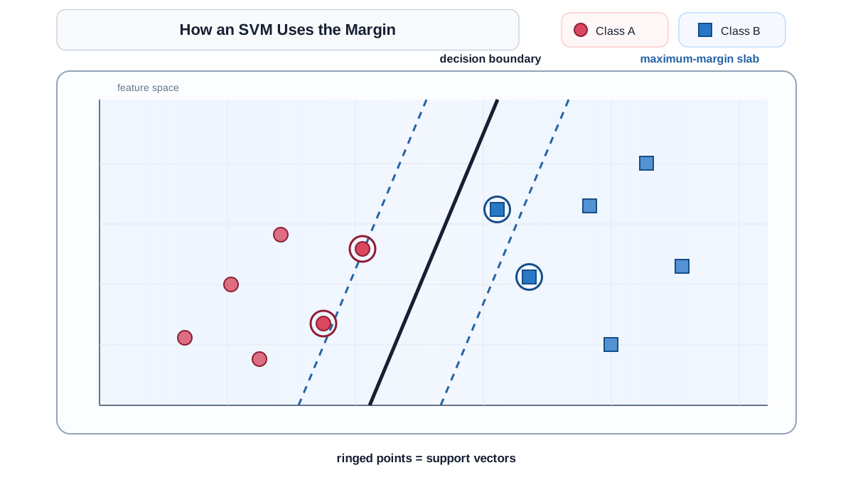
Picture two clusters of points on a flat sheet of paper—red on the left, blue on the right. Your job is to draw a straight line that separates them. There are infinitely many lines that will do the job. Some cut close to the red cluster. Some hug the blue cluster. Most of them work perfectly on the points you already have, and most of them will feel fragile the moment new points arrive.

The support vector machine asks a sharper question: of all the lines that separate the classes, which one leaves the most room on both sides?

That room is the margin. Formally, the margin is the widest empty slab you can place between the two classes, parallel to your separating line. The SVM finds the line that maximizes that slab's width. A wider margin means the boundary is not balanced on a knife's edge—small movements in the data are less likely to flip a prediction to the wrong side.

Here is the part that surprises most beginners. In this clean, perfectly separable picture, the points sitting far from the boundary contribute nothing to the fit. The boundary is held in place by the few points that touch the edges of the slab. Those edge-touching points are the support vectors.

But do not take that literally for every SVM you fit. The clean picture I just described is the hard-margin case, where the data separates perfectly and only the edge points matter. Real SVMs use soft margins and kernels, which change the story: points that fall inside the margin or on the wrong side can also become support vectors, and with a flexible kernel the support vector set can grow large. The durable idea is not "SVMs use almost no data." It is that the model's decision boundary is defined by the training examples that sit closest to the fight—not by the bulk of points safely on one side.

This is why SVMs are memory-efficient in a way many models are not. The decision function—the score the model computes to choose a side for a new point—depends only on the support vectors, not on your full dataset. In scikit-learn, you can inspect support_vectors_ after fitting an SVC and see exactly which points earned that role.

Common mistake: Assuming the SVM uses all your data to make predictions. It does not. But do not assume support vectors are always a tiny, tidy subset either. In soft-margin and kernel SVMs, they can include points inside or across the margin.

Hard Margins, Soft Margins, and the C Tradeoff

The clean two-cluster picture has a problem: real data is rarely that tidy. Classes overlap. Noise sneaks in. A single stray point from the red class can sit deep in blue territory, and suddenly no straight line can separate the classes perfectly.

A hard-margin SVM demands perfect separation. It will contort itself to find a line that puts every training point on the correct side. When your data contains noise, that demand produces a boundary that winds around outliers, memorizes the training set, and generalizes poorly to anything new.

The fix is the soft margin. Instead of requiring every point to be on the correct side, the soft-margin SVM allows some points to violate the boundary—in exchange for a wider, more honest margin overall. The tradeoff is controlled by a single parameter, C.

Think of C as a dial between two failure modes:

• Low C: You tolerate more training errors in exchange for a wide, simple margin. The model generalizes better but may underfit if the data has real structure you are ignoring.
• High C: You punish training errors harshly. The model fights to classify every point correctly, which means it will chase noise and outliers. High C is the overfitting zone.

The name "C" comes from the optimization formulation, where it acts as a penalty weight on misclassified points. In scikit-learn's SVC, you set it directly. A reasonable first experiment is to start with C somewhere in the middle—say, 1.0—and then move it in powers of ten while watching validation performance.

Warning: C is not the only knob. Once you introduce kernels, a second parameter called gamma enters the picture, and the two interact. Tuning C while ignoring gamma is like adjusting the volume on a stereo while someone else keeps changing the balance.

The Kernel Trick: Curved Boundaries Without Leaving 2D

Some datasets simply cannot be separated by a straight line. Imagine blue points forming a ring around a central cluster of red points. No line will ever separate them. You could draw a circle, but a linear classifier has no vocabulary for circles.

The classic workaround is to add a feature. What if, alongside your original coordinates, you gave each point a third value: its distance from the origin? In that new three-dimensional space, the ring and the central cluster suddenly separate cleanly—the ring points have large distances, the central points have small ones. A flat plane in 3D does what no line could do in 2D.

That is the conceptual core of the kernel trick. The SVM does not actually add features and compute in a higher-dimensional space. It uses a mathematical shortcut—the kernel function—that computes the similarity between points as if they had been transformed, without ever building the transformed space. The result is that a linear algorithm draws curved boundaries in your original space.

Three kernels cover most practical work:

Kernel	What it assumes	When to reach for it
Linear	Classes separate by a straight boundary	High-dimensional data, text features, many features with few samples
Polynomial	Boundary follows a polynomial curve	Rarely the best default; useful when you have domain reason to expect polynomial structure
RBF (radial basis function)	Boundary can be any smooth curve	A common baseline for non-linear problems; flexible, but it needs tuning and validation

The RBF kernel introduces gamma, which controls how local each training point's influence is. Low gamma means each point influences a wide neighborhood, producing a smooth, simple boundary. High gamma means each point influences only its immediate surroundings, producing a boundary that can twist tightly around individual points. High gamma is the overfitting dial for kernels.

You do not need the derivation to use kernels well. You need the mental model: the kernel is a similarity measure that lets the SVM find curved separations by pretending it is working in a space where the data is linearly separable.

Scaling, Tuning, and the Practical Cost of SVMs

SVMs are geometry-based models. The margin is measured in the feature space, and the kernel compares points by their proximity. If one feature ranges from 0 to 1 and another ranges from 0 to 100,000, the second feature dominates every distance calculation, and the first becomes irrelevant.

This is why feature scaling is non-negotiable. Standardize or normalize your features before fitting an SVM, or the model will quietly ignore most of your data. If you have worked with K-nearest neighbors, the reason will feel familiar: both models live and die by distance.

The tuning burden is real. C and gamma interact, which means you cannot tune them independently. The standard workflow is a grid search over both, typically on a logarithmic scale. In scikit-learn, GridSearchCV over C and gamma values like [0.01, 0.1, 1, 10, 100] is a conventional starting point. This is not a one-shot fit; it is a small experiment loop.

There is a workflow trap hiding here. If you scale your features before running cross-validation, the scaler learns statistics from the full dataset—including your validation folds. That leaks information and gives you an optimistic score. The fix is to put the scaler inside a scikit-learn Pipeline along with the SVM, so each training fold learns its own scaling statistics and applies them to its own validation fold. This is the same leakage discipline you need for any distance-based or regularized model.

Training cost is another constraint. The SVM optimization scales poorly with sample count—roughly quadratically in the number of training examples for the standard implementation. On a few thousand points, training is instant. On hundreds of thousands, it becomes slow enough that you will feel it. On millions, you will look for another tool.

There is also the probability problem. An SVM produces a decision score—a signed distance from the boundary—not a calibrated probability. A point far from the boundary gets a large score, but that score does not mean the model is 95 percent certain in the way logistic regression's output does. scikit-learn offers probability=True, which fits an additional calibration stage to convert scores into probability-like values, but that costs extra computation and the result is not as reliable as what logistic regression gives you natively. If your workflow depends on trustworthy probabilities for thresholding or risk scoring, an SVM is working against you.

When to Reach for an SVM (and When Not To)

The honest summary is that SVMs are a precision tool, not a universal default. They shine when your problem has a clear boundary, your dataset is moderate in size, and your feature space is rich enough that a linear model underfits but a tree ensemble feels like overkill.

Here is the decision frame I use:

Reach for an SVM when: you have a clean, moderately sized dataset (up to tens of thousands of samples), a non-linear boundary is likely, and you have already scaled your features. Text classification with many features is a classic sweet spot, as are problems where the number of features exceeds the number of samples.

Look elsewhere when: your dataset is very large, you need interpretable coefficients, or you need calibrated probabilities. For those cases, a linear model gives you speed and interpretability, and a tree ensemble like a random forest or gradient boosting handles scale and feature interactions without demanding scaling.

What about heavy class overlap? Do not rule out SVMs on that basis alone—soft margins exist precisely to handle overlap. The better test is whether cross-validation shows the SVM generalizing better than a simpler baseline. If a linear model or a small tree ensemble matches its performance with less tuning, the SVM's extra flexibility is not earning its keep.

Against logistic regression, the SVM offers more flexibility through kernels but gives up calibrated probabilities and clean coefficient interpretation. Against tree ensembles, the SVM often wins on small, high-dimensional, clean problems but loses on large datasets and lacks a built-in feature-importance story.

The geometric mental model is the durable takeaway. Even if you rarely deploy an SVM in production, understanding margins and support vectors changes how you think about every other classifier. It teaches you that the points near the boundary are the ones that matter, that a wide margin means a more stable boundary—not a guarantee of correctness—and that a model's complexity is a dial you control, not a property you inherit.

Try it yourself. Take a small, clean dataset—the iris data with two classes works well. Build a scikit-learn Pipeline that scales the features and fits an RBF SVM with C=1 and gamma=0.1, then compare it against a pipeline with a linear baseline. Run cross-validation on both. Move C up and down. Move gamma. Watch the validation score follow. The model stops being a black box the moment you see which points hold it in place—and which ones you let cross the line.

References

Research updated Sep 8, 2026