Support Vector Machines: Derive the Maximum-Margin Classifier

Most explanations of support vector machines stop at the picture: two clouds of points, a line between them, a gap on either side. That picture is correct, and it is also useless the moment you need to know why changing one number flips a boundary, why only a handful of training points matter, or why unscaled features quietly wreck the result. The picture describes the answer. It does not describe the problem.

This article writes the problem down. We will build the maximum-margin classifier from a raw geometric goal into a constrained optimization objective, then relax it so it survives real, overlapping data. By the end you should be able to read any SVM formulation and name three things: its objective, its constraints, and its price of violation.

If margins, support vectors, and kernels are still fuzzy, the intuition-level treatment of margins and kernels is the right place to start. Here we assume you know what a margin looks like and want the mathematics behind it.

Notation and the Geometry We Are Optimizing

Fix the symbols first, because every later equation depends on them.

We have a dataset of $n$ samples. Each input is a vector $x_i \in \mathbb{R}^d$, and each label is $y_i \in \{-1, +1\}$. The two-class encoding matters: using $-1$ and $+1$ instead of $0$ and $1$ lets a single expression handle both classes.

A linear classifier is a hyperplane:

$w^T x + b = 0$

Here $w \in \mathbb{R}^d$ is the normal vector — it points perpendicular to the hyperplane and sets its orientation. The scalar $b$ is the bias, which shifts the hyperplane away from the origin.

The quantity $w^T x_i + b$ is a signed score. Its sign tells you which side of the hyperplane the point falls on, and its magnitude grows with distance from the boundary. To convert that score into an actual distance, divide by the length of the normal vector:

$\text{signed distance} = \frac{w^T x_i + b}{\|w\|}$

The sign still encodes the predicted side. Multiply by the true label $y_i$, and you get a quantity that is positive when the point is correctly classified and negative when it is not:

$y_i(w^T x_i + b)$

This is the functional margin for a single point. It is positive on the correct side, and its size depends on the scale of $w$ and $b$.

That last clause is the hinge the whole derivation turns on. Multiply $w$ and $b$ by any positive scalar and you get the same hyperplane — same orientation, same position, same predictions. The boundary is scale-invariant. The functional margin is not. This mismatch is not a bug to work around; it is the freedom we will spend to make the problem clean.

From "Widest Street" to a Constrained Objective

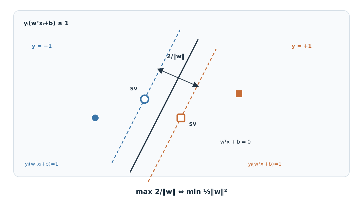
Start from the raw goal, stated without symbols: find the hyperplane that correctly separates the two classes and sits as far as possible from the nearest point of either class.

Two requirements are tangled together here. First, every point must land on the correct side: $y_i(w^T x_i + b) > 0$ for all $i$. Second, the distance from the hyperplane to the closest point — the geometric margin — must be as large as possible.

Written directly, that objective is awkward:

$\max_{w, b} \frac{1}{\|w\|} \min_i \left| w^T x_i + b \right| \quad \text{subject to} \quad y_i(w^T x_i + b) \geq 0$

A minimum nested inside a maximum, with an absolute value, is unpleasant to optimize. The scale-invariance rescues us.

Because scaling $w$ and $b$ does not change the hyperplane, we are free to choose the scale. So choose the convenient one: fix the functional margin of the closest points to exactly $1$. Concretely, require

$y_i(w^T x_i + b) \geq 1 \quad \text{for all } i$

This single constraint does two jobs at once. It enforces correct classification, because the left side is positive. And it pins down the scale, because the closest points now sit at a functional margin of exactly $1$.

With the scale fixed, the geometric margin has a clean value. The two margin boundaries sit at $w^T x + b = +1$ and $w^T x + b = -1$. The distance between them is

$\frac{2}{\|w\|}$

So maximizing the margin means maximizing $2/\|w\|$, which means minimizing $\|w\|$. Squaring and halving changes nothing about where the minimum sits, but it gives a friendlier derivative:

$\min_{w, b} \frac{1}{2}\|w\|^2 \quad \text{subject to} \quad y_i(w^T x_i + b) \geq 1, \quad i = 1, \dots, n$

This is the hard-margin primal problem. The objective is convex and quadratic; the constraints are linear. That combination buys something specific: when the data is linearly separable, the solution is unique. There is exactly one widest street, and this problem finds it.

Note: The jump from "maximize the margin" to "minimize $\|w\|$" is where most derivations lose people. The step is not a trick. It is the direct consequence of fixing the functional margin to $1$ and then measuring the real distance with $\|w\|$ in the denominator.

Why Only Some Points Matter: Support Vectors and KKT

The constraint set has $n$ inequalities, one per training point. You might expect all $n$ to influence the answer. They do not, and the reason is the structure of constrained optimization.

Attach a Lagrange multiplier $\alpha_i \geq 0$ to each constraint and form the Lagrangian. Solving it produces a condition known as complementary slackness, one of the Karush-Kuhn-Tucker (KKT) conditions:

$\alpha_i \left[ y_i(w^T x_i + b) - 1 \right] = 0$

Read this literally. The product is zero, so at least one factor must be zero.

• If a point sits strictly outside the margin, then $y_i(w^T x_i + b) > 1$, the bracket is positive, and therefore $\alpha_i = 0$.
• If a point sits exactly on the margin, then $y_i(w^T x_i + b) = 1$, the bracket is zero, and $\alpha_i$ is free to be positive.

Points with $\alpha_i > 0$ are the support vectors. They are the only points that appear in the final decision function, which is a weighted sum over them:

$f(x) = \text{sign}\left( \sum_{i \in SV} \alpha_i y_i \, x_i^T x + b \right)$

Everything else has been multiplied by zero and dropped.

A Three-Point Example

Take three points in two dimensions. Two sit exactly on the margin boundaries — one at $w^T x + b = +1$, one at $w^T x + b = -1$. The third sits far away on the correct side.

The two margin points have tight constraints, so their brackets are zero and their $\alpha_i$ can be positive. The distant point has a loose constraint, so its bracket is positive and its $\alpha_i$ must be zero. The decision boundary is defined entirely by the two margin points. Move the distant point anywhere on its side of the boundary and nothing changes. Move either margin point and the boundary shifts.

That is the formal reason SVMs are memory-efficient at prediction time: the model stores the support vectors, not the dataset.

The Dual Problem and Why It Sets Up Kernels

The primal problem is solvable, but its dual form exposes something more useful. Substituting the stationarity conditions back into the Lagrangian yields the dual objective:

$\max_{\alpha} \sum_i \alpha_i - \frac{1}{2} \sum_{i,j} \alpha_i \alpha_j y_i y_j \, x_i^T x_j$

subject to

$\sum_i \alpha_i y_i = 0, \qquad \alpha_i \geq 0$

Look at where the data appears. Every input vector shows up only inside the inner product $x_i^T x_j$. Nowhere else. Not as a coordinate, not as a feature, only as a pairwise similarity.

That structural fact is the precondition for the kernel trick. If the algorithm depends on the data only through inner products, you can replace the inner product with a kernel function:

$x_i^T x_j \;\longrightarrow\; K(x_i, x_j)$

The kernel computes the inner product in some richer representation without ever materializing coordinates in that space. A polynomial kernel, a radial basis function kernel, and others each define a different geometry of decision surface.

Be precise about what this buys you. A kernel changes the representation and therefore the shape of the boundary the model can express. It does not guarantee better generalization. A kernel that matches the structure of your data can help substantially; a poorly matched one can hurt, and it adds hyperparameters you now have to tune. The kernel trick is a change of geometry, not a promise of accuracy.

Soft Margins: When the Data Refuses to Separate

The hard-margin problem assumes a separating hyperplane exists. Real data often refuses. When classes overlap, the constraint set has no feasible solution at all. When they barely separate, a single mislabeled point can drag the boundary into a bad position, because that point becomes a support vector and the margin must accommodate it.

The fix is to let points violate the margin, but charge them for it. Introduce slack variables $\xi_i \geq 0$, one per point, measuring how far that point violates the margin:

$y_i(w^T x_i + b) \geq 1 - \xi_i$

A point with $\xi_i = 0$ respects the margin. A point with $0 < \xi_i < 1$ sits inside the margin but on the correct side. A point with $\xi_i \geq 1$ is misclassified. Now add the total violation to the objective, scaled by a parameter $C$:

$\min_{w, b, \xi} \frac{1}{2}\|w\|^2 + C \sum_i \xi_i \quad \text{subject to} \quad y_i(w^T x_i + b) \geq 1 - \xi_i, \quad \xi_i \geq 0$

This is the soft-margin primal. The parameter $C$ is the price of violation.

• Large $C$ punishes violations hard. The model pushes toward a narrow margin with few errors.
• Small $C$ tolerates violations. The model widens the margin and accepts more points inside it.

In the dual, the only change is an upper bound on each multiplier: $0 \leq \alpha_i \leq C$. That bound is worth pausing on. It caps how much influence any single training point can have on the boundary. Under the hard-margin problem, one outlier could pull with unlimited force. Under the soft-margin problem, its pull is capped at $C$.

There is a second way to read the same objective. The soft-margin problem is equivalent to minimizing

$\frac{1}{2}\|w\|^2 + C \sum_i \max\left(0, 1 - y_i(w^T x_i + b)\right)$

The term $\max(0, 1 - z)$ is the hinge loss. It is zero once a point is correctly classified and outside the margin, and it grows linearly as the point moves toward and past the boundary. This connects the SVM to the loss-function view you have already seen for other linear models: a data-fit term plus a regularization term, traded off by a single constant.

That constant is not derived from the data. $C$ is a hyperparameter, tuned by validation.

What the Derivation Predicts About Real Behavior

The mathematics is not decoration. It predicts specific failure modes, and knowing them saves debugging time.

Feature scaling is not optional. The margin depends on $\|w\|$ and on distances measured in feature space. If one feature ranges over thousands and another over fractions, the constraint set is dominated by the large-scale dimension. The model will effectively ignore the small one. This is a direct consequence of the geometry, not a quirk of any library. Standardize your features before fitting.

Outlier sensitivity depends on which margin you chose. Hard-margin SVMs are fragile: one point inside the margin can make the problem infeasible or distort the boundary badly. Soft-margin SVMs absorb that point through its slack variable and cap its influence at $C$. If your data has noise or label errors — and it does — you want the soft-margin formulation.

The number of support vectors is a rough complexity signal. More support vectors means more points are pressing against the margin, which usually means a more complex boundary. Lowering $C$ tends to increase the support-vector count and widen the margin; raising it does the opposite. Watching that count as you tune $C$ gives you a readable signal of what the model is doing.

When the derivation says an SVM is a reasonable choice: moderate sample sizes, high-dimensional or sparse representations, and problems where a clear margin is plausible. The method was built for exactly those conditions.

When it is not: very large datasets, where the underlying quadratic program becomes the bottleneck, or problems where calibrated probabilities and direct coefficient interpretation matter more than the boundary itself. An SVM gives you a decision, not a probability, and its support-vector expansion is not a coefficient table you can read like linear regression.

Where to Take This Next

You now have the full chain: geometry to functional margin, functional margin to normalized constraint, constraint to primal objective, primal to dual, dual to kernels, and hard margin to soft margin with slack and $C$.

The way to make it stick is to rebuild it from memory. Write the hard-margin primal on a blank page — objective, constraints, and the reason the constraint is normalized to $1$. Then re-derive the soft-margin version by adding slack variables and the penalty term. If you can do both without looking, you understand the model rather than recognizing it.

Then run the check that turns theory into evidence. Fit a linear SVM on a small dataset, pull out the support vectors, and compare them against the KKT condition: which points have nonzero multipliers, and do they sit on or inside the margin? The points the solver hands back should match the ones the complementary slackness condition predicted. When they do, the derivation stops being algebra and becomes something you can see in the output.