
Derive the Poisson Regression Objective With a Log Link
A straight line on count data will eventually promise you a negative number of events. The Poisson likelihood with a log link is what stops it.

Key topics
A straight line on count data will eventually promise you a negative number of events. The Poisson likelihood with a log link is what stops it.
Why Counts Need Their Own Objective
Suppose you are modeling the number of support tickets a customer files in a month, the number of failures a machine logs per shift, or the number of purchases a visitor makes in a session. Your target lives on : non-negative integers, usually with a pile of zeros and a long right tail.
Ordinary least squares does not respect that support. Fit a line to counts and, for some feature values, the predicted mean drops below zero. A negative expected count is not a small numerical annoyance; it is a statement that cannot be true. OLS also assumes the noise has constant variance, but counts rarely behave that way — when the mean count is large, the spread tends to be large too.
The obvious patch is to log-transform the raw counts and run OLS on . It fails the moment a single observation is zero, because is undefined. Adding one before the log keeps the code running, but now you are fitting a different model than the one you described, and the coefficients no longer mean what you think they mean.
The real fix is not to transform the data. It is to model the mean through a link function and let the distribution handle the integer support. That is the generalized linear model move, and the Poisson case is the cleanest place to see it work.
Note: If the linear predictor, link function, and response distribution split still feels abstract, treat this article as the concrete instance. Everything here is one specific choice of distribution and one specific choice of link.
Notation and the Two Modeling Choices
Before any derivation, pin down the symbols.
We observe pairs for . Here is a realized count and is a feature vector for observation . The parameters are a coefficient vector , which includes an intercept. The linear predictor is
This quantity is unbounded: it can be any real number. That is the whole tension. Counts are non-negative integers; linear predictors are unrestricted reals. Two independent decisions bridge the gap.
Choice 1 — the response distribution. We assume
with probability mass function
The Poisson family already lives on the correct support. Its single parameter is both the mean and the variance, a fact we will return to when we discuss assumptions.
Choice 2 — the link. We connect the mean to the linear predictor with
Why the log? Two reasons. First, maps any real number to a strictly positive one, so the predicted mean can never go negative no matter what or do. Second, the log is the canonical link for the Poisson family — the one that falls out of writing the Poisson PMF in exponential-family form. Canonical links tend to produce well-behaved, convex objectives, which is exactly what we will find.
We also assume the observations are independent given the features. The likelihood is a product, and that product only factors cleanly under independence.
Knowledge check
Check your understanding
Answer this question before you continue.
From the Poisson PMF to the Likelihood
Start with a single observation. Its contribution to the likelihood is just the PMF evaluated at the observed count:
Now substitute the link. Since , the PMF becomes a function of :
Independence lets us multiply these contributions across all observations. The likelihood is
This is the count regression likelihood in its raw form. Notice that the terms do not contain at all. They are constants with respect to the parameters, so they will drop out of any optimization. That is why most treatments write the objective without them.
Knowledge check
Check your understanding
Answer this question before you continue.
Taking the Log: The Objective You Actually Optimize
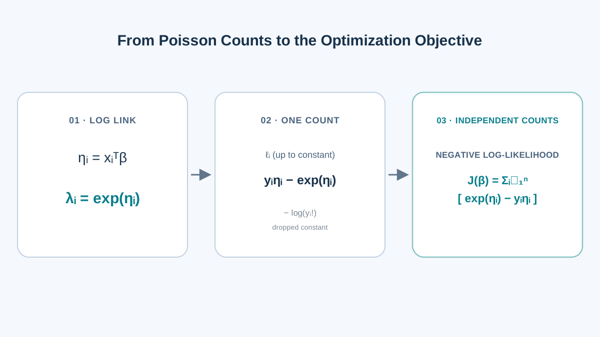
Products of many small probabilities underflow fast, and differentiating a product is painful. Take the natural log. The product becomes a sum:
where I have written for to keep the line readable. Drop the -free constant and you have the log-likelihood up to an additive constant:
Solvers minimize rather than maximize, so flip the sign to get the negative log-likelihood:
Two terms are doing all the work, and each has a clear job.
- rewards pushing the linear predictor up when the observed count is large. A big makes the model want a big .
- penalizes large predicted means regardless of what was observed. Even when is zero, this term pulls down.
The two terms fight, and the balance point is not where each prediction equals its observed count. It is where the feature-weighted residuals balance across the whole dataset. To see why, differentiate the objective with respect to and set the gradient to zero:
Read that equation carefully. Each observation contributes a residual , weighted by its feature vector . At the optimum, those weighted residuals cancel out across the dataset. A single observation with and is not forced to match; it is balanced against every other observation through the shared . The model trades off errors across all rows to satisfy one aggregate condition per coefficient.
That is the mechanism behind every fitted Poisson model: not per-point matching, but a joint, feature-weighted compromise.
One more property matters in practice: this objective is convex in . There is a single global optimum and no local-minimum trap. It is a large part of why Poisson GLMs are so easy to fit reliably.
Knowledge check
Check your understanding
Answer this question before you continue.
Worked Example: One Observation, One Feature
Numbers make the algebra concrete. Take a single observation with and , and a candidate , where the first entry is the intercept.
Compute the linear predictor:
Convert to the mean:
Evaluate the single-observation log-likelihood term:
Change slightly and the value moves. That surface — one number per candidate parameter vector — is what the solver walks downhill.
You can verify the same quantity in code. The negative log-likelihood for a fitted model is a direct translation of the formula:
import numpy as np
from scipy.special import gammaln

def poisson_nll(beta, X, y):
    eta = X @ beta
    # gammaln(y + 1) == log(y!) but stable for large counts
    return np.sum(np.exp(eta) - y * eta + gammaln(y + 1))
Fit a PoissonRegressor from scikit-learn on a small count dataset, then plug the fitted coef_ and intercept_ into this function. The value you compute by hand should match the model's reported log-likelihood up to sign. When it does, you have confirmed that the derivation and the library are solving the same problem.
Common mistake: Comparing a hand-computed log-likelihood to a library's reported value without checking whether the library includes the constant. Some report the full log-likelihood; some report it up to a constant. The difference is a fixed offset, not a modeling error.
Reading the Coefficients: Multiplicative Effects
Because , a one-unit increase in feature adds to the log of the expected count. Exponentiating, it multiplies the expected count by .
| Coefficient | Effect on the expected count |
|---|---|
| No change in the rate | |
| Count grows by a factor of | |
| Count shrinks by a factor of |
This is the same log-to-odds move you already know from logistic regression, except the quantity being scaled is a rate rather than a probability. In epidemiology and economics, is often called an incidence rate ratio.
When counts come from windows of different sizes — different observation periods, different populations — you add to the linear predictor with a fixed coefficient of 1. This is an offset, and it turns the model into a rate model: you are now predicting events per unit of exposure rather than raw counts.
Assumptions and Where the Model Breaks
The derivation is clean, but it rests on assumptions that real data violates constantly.
Mean equals variance. The Poisson family forces . Real count data is frequently overdispersed: the variance exceeds the mean. Overdispersion inflates standard errors and makes the model look more confident than the evidence supports. Negative binomial or quasi-Poisson models are the usual escapes.
Independence. The product likelihood assumes observations do not influence each other. Clustered or repeated-measures data violates this, and the standard errors will be wrong even if the coefficients look reasonable.
Multiplicative structure. The log link assumes effects compound multiplicatively on the mean. That is a strong structural claim, not a neutral default. If your domain expects additive effects, the log link will fight you.
Excess zeros. If your data has more zeros than the Poisson predicts, a plain Poisson fit will be biased. Zero-inflated or hurdle models are the right tool.
Warning: Convexity guarantees a unique optimum. It says nothing about whether the Poisson distribution is the right description of your data. A perfectly fitted wrong model is still wrong.
Knowledge check
Check your understanding
Answer this question before you continue.
When to Reach for This Model
Use Poisson regression when the target is a non-negative integer count and the mean-variance relationship is roughly Poisson. Prefer it over OLS on counts whenever negative predictions or heteroscedasticity would distort the fit. Prefer it over log-transformed OLS when zeros are present or when you want a principled likelihood rather than an ad hoc transform.
Move to negative binomial, zero-inflated, or hurdle variants when diagnostics point to overdispersion or excess zeros. The derivation you just worked through is the foundation those models extend.
Next Step
Fit a PoissonRegressor on a small count dataset. Compute the negative log-likelihood by hand for the fitted coefficients using the formula above, and compare it to the model's reported value. Then check the mean-variance relationship in the residuals: if the variance clearly exceeds the mean, that is your signal to look at overdispersed alternatives next.
Knowledge check
Final check
Finish the article by checking the ideas you just learned.
References
Build stronger machine learning foundations
Use structured resources to connect theory, scikit-learn workflows, and evaluation practice.


