
Quantile Regression: Derive the Pinball-Loss Objective
Your model keeps under-predicting the values you actually care about, and averaging the errors away does not fix it.

Key topics
Your model keeps under-predicting the values you actually care about, and averaging the errors away does not fix it.
That is the symptom. The cause is usually a quiet assumption buried in the loss function: squared error decides that the thing worth predicting is the conditional mean. If your real cost is asymmetric — a missed high demand hurts more than an overstocked shelf — then you are optimizing the wrong functional of the distribution. This article derives the objective that fixes it, from the asymmetry up, so you can regenerate the formula instead of memorizing it.
Why the Mean Is the Wrong Target
Picture a supply planner. Under-predicting demand means empty shelves and lost sales. Over-predicting means warehouse cost and markdowns. Those two errors do not cost the same, yet a model trained on squared error treats a +10 miss and a −10 miss as identical. It will happily sit in the middle of the conditional distribution, which is exactly where the expensive errors live.
The mean is a summary, not a universal target. When the conditional distribution is skewed or heavy-tailed, the mean can sit in a region where almost no observation actually lands. You get a number that minimizes average squared distance and answers a question nobody asked.
Here is the reframe that matters: a loss function is not a scoreboard bolted on after training. It is the definition of what the model is trying to estimate. Squared error buys you the conditional mean. Absolute error buys you the conditional median. An asymmetric absolute error buys you a conditional quantile. Change the loss, and you change the target — not just the score.
If you have already worked through least-squares fitting and residuals, you have the machinery. We are changing the objective, not the fitting.
Notation and the Quantile Function
Before the derivation, pin down every symbol.
- : the input vector.
- : the target.
- : the prediction.
- : the quantile level.
- : the conditional CDF of given .
The -quantile of the conditional distribution is the smallest value such that . When the CDF is continuous and strictly increasing, this is simply the value where . When the CDF has jumps — a discrete or degenerate distribution — the quantile is a set, and we will come back to that.
The distinction that trips people up: an unconditional quantile is one number for the whole sample. A conditional quantile is a function of . That function is the object a quantile regression model estimates. Two different inputs can have two different 90th percentiles, and the model is supposed to capture that.
One assumption to state plainly: the derivation below is a population statement about the true conditional distribution. It says what the loss is minimized by in the limit of infinite data. It is not a guarantee about a finite fitted model.
Knowledge check
Check your understanding
Answer this question before you continue.
Building the Pinball Loss From the Asymmetry
Start from absolute error, , and ask what happens if you weight the two sides differently. Weight under-prediction by and over-prediction by :
The compact form is the same object:
Check the boundary case. At , both branches carry weight , so the loss is half the absolute error and the minimizer is the median. The median is not a separate method; it is the special case.
Geometrically, this is a kinked, asymmetric V. The kink sits at , and the two arms have different slopes. That asymmetry is the whole mechanism: the optimizer slides toward whichever side is penalized more steeply until the two forces balance.
You will see this called the pinball loss, the quantile loss, and the check function. Same object, different names across papers and libraries.
Knowledge check
Check your understanding
Answer this question before you continue.
Deriving the Minimizer: Why the Optimum Is the Quantile
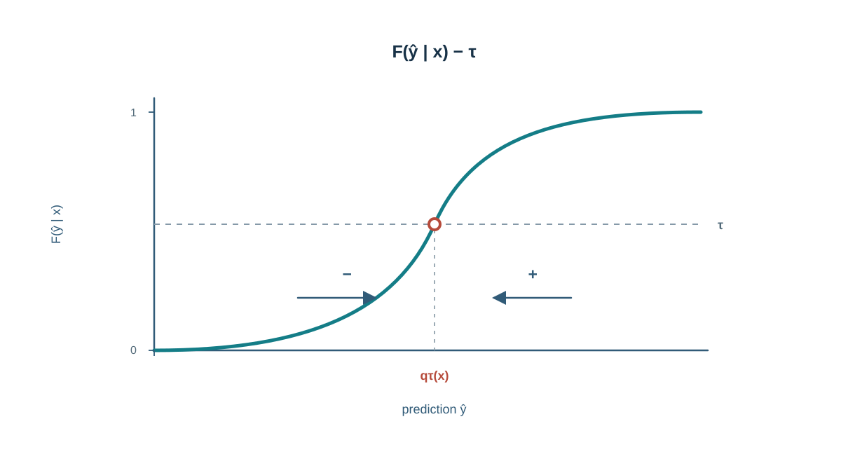
Now the actual derivation. Fix and consider the expected loss over :
Differentiate with respect to . The first integral contributes ; the second contributes . Collect:
Set it to zero:
The population minimizer is the value where the conditional CDF crosses — the -quantile.
Read the derivative's sign on either side and the behavior becomes obvious. Below the quantile, , so the gradient is negative and pushes the prediction up. Above it, the gradient is positive and pushes down. The equilibrium is exactly where the CDF crosses .
In plain causal language: when , under-prediction is steeper, so the optimizer drifts upward until roughly of the probability mass sits below the prediction. That is the asymmetry doing its job.
What breaks when assumptions fail? If the conditional distribution is discontinuous or degenerate, jumps over and the minimizer is a set of values rather than a unique point. Finite-sample fits inherit that ambiguity — you may see the loss surface flat over a range.
Knowledge check
Check your understanding
Answer this question before you continue.
A Worked Example You Can Check by Hand
Take a tiny fixed sample: . Try and evaluate the pinball loss at a few candidate predictions. For each candidate, split the points into under-predictions (, weighted by ) and over-predictions (, weighted by ).
| Under-predictions | Over-predictions | Loss at | |
|---|---|---|---|
| 3 | — | ||
| 4 | |||
| 10 |
The minimum lands on the sample 90th quantile, which for five points is the largest value, 10. The asymmetry is visible in the table: at every point is an under-prediction and the steep weight dominates; at every point is an over-prediction and the shallow weight keeps the total small. Now repeat at and the minimum lands on the median, 3 — the MAE special case.
You can verify the sweep in a few lines:
import numpy as np

y = np.array([1, 2, 3, 4, 10])
candidates = np.arange(0, 12, 0.5)

def pinball(y, yhat, tau):
    return np.mean(np.where(y >= yhat, tau * (y - yhat),
                            (1 - tau) * (yhat - y)))

for tau in (0.5, 0.9):
    losses = [pinball(y, c, tau) for c in candidates]
    print(tau, candidates[int(np.argmin(losses))])
The output confirms the algebra: the loss curve is asymmetric, and its lowest point is not the mean.
Reading the Quantile Level as a Lever
is not a confidence level. It is the fraction of the conditional distribution expected to fall at or below the prediction. At , you are saying: about 90% of the mass sits below this value.
Fit several values and you trace out the shape of the conditional distribution. Spread, skew, and heteroscedasticity become visible instead of being averaged away. If the conditional spread widens with , a single mean model hides it; a fan of quantile models exposes it.
Choose from the cost ratio between over- and under-prediction, not from a default. If a miss high costs three times a miss low, the ratio points you toward a above 0.5.
Knowledge check
Check your understanding
Answer this question before you continue.
What Quantile Prediction Does Not Guarantee
This is where the expensive mistake lives. Stack a 0.1 model and a 0.9 model and you get an interval-shaped output. Nothing in the pinball objective enforces 80% coverage.
Coverage is a property of the joint behavior of both quantile estimates plus the data distribution. Each quantile can be individually well-fit and the pair can still miscover. Worse, independently fitted quantiles can invert — the 0.1 prediction lands above the 0.9 prediction, producing a negative-width interval. That is quantile crossing, and it is a symptom of fitting each level in isolation.
The population result is asymptotic. A flexible model can fit the training quantiles without generalizing the coverage.
Common mistake: reading a quantile pair as a calibrated interval. Measure empirical coverage on held-out data, and treat calibration as a separate step rather than a byproduct of the loss.
When to Reach for Quantile Regression
Use it when the cost of error is asymmetric, when the conditional spread matters, or when the mean is a poor summary of a skewed target. Skip it when a symmetric loss matches the real cost, when you need a single point estimate, or when you need guaranteed coverage and have not budgeted for calibration.
There is a robustness angle worth noting: because the loss grows linearly rather than quadratically, extreme targets exert less pull on the fit than they would under squared error. That is a feature when outliers are noise and a liability when they are signal.
This article derived the objective. The estimator, solver, and tuning choices are a separate topic.
The One-Line Result, and What to Do With It
The pinball loss is minimized by the conditional quantile. That is the whole derivation compressed into a sentence.
Turn it into a decision rule: choose from the cost asymmetry, fit several quantiles to see the conditional spread, and never read a quantile pair as a calibrated interval without measuring coverage.
Here is your next move. Pick one skewed target you already have. Fit a median model and a high-quantile model, then compute empirical coverage on held-out data against the nominal level. The gap you see is the difference between predicting a quantile and owning an interval — and it is the gap that separates a model that looks right from one that survives contact with a real decision.
Knowledge check
Final check
Finish the article by checking the ideas you just learned.
References
Build stronger machine learning foundations
Use structured resources to connect theory, scikit-learn workflows, and evaluation practice.


