Least-Squares Linear Regression: Derive the Objective and Solution

Call LinearRegression().fit(X, y) and coefficients appear in milliseconds. The library never shows you the equation it solved, why that equation has a closed-form answer, or when the answer stops being trustworthy. This article reads the machine's source code: the objective, the derivative, the normal equations. By the end, those coefficients stop being magic numbers and become consequences of a specific minimization problem.

If you have already seen the intuition — a line through points, residuals as vertical gaps — you are ready. We are going to name the quantity being minimized, then solve for it exactly.

What the Solver Is Actually Minimizing

For a single data point, the residual is the difference between the observed value and the model's prediction:

$e_i = y_i - \hat{y}_i$

A positive residual means the model predicted too low; a negative one means too high. If we summed raw residuals, a large positive miss and a large negative miss would cancel, and a line that is badly wrong in both directions could look perfect. So we square each residual before summing. The result is the residual sum of squares, also called the least-squares objective function:

$\text{RSS}(w) = \sum_{i=1}^{n} \left(y_i - \hat{y}_i\right)^2$

Squaring does three useful things. It removes sign cancellation. It penalizes large misses far more than small ones — a residual of 4 contributes 16, while four residuals of 1 contribute only 4. And it produces a smooth, differentiable curve, which is what makes the closed-form solution possible.

The prediction itself is a weighted sum of features plus an intercept:

$\hat{y}_i = w_0 + w_1 x_{i1} + w_2 x_{i2} + \cdots + w_d x_{id}$

The weights $w_0, w_1, \ldots, w_d$ are the unknowns. Everything else — the $x$ values and the $y$ values — is data we already have.

Note: Minimizing squared error is a choice, not a law of nature. It encodes a preference for small errors and a strong sensitivity to outliers. A single point far from the pack can drag the whole line toward it, because its squared residual dominates the sum.

Notation: Design Matrix, Parameter Vector, Residual Vector

Writing the sum for every point gets unwieldy fast. Matrix notation compresses it into one expression and makes the derivative tractable.

Stack the data into a design matrix $X$ with one row per example and one column per feature. Add a leading column of ones to carry the intercept:

$X = \begin{bmatrix} 1 & x_{11} & \cdots & x_{1d} \\ 1 & x_{21} & \cdots & x_{2d} \\ \vdots & \vdots & \ddots & \vdots \\ 1 & x_{n1} & \cdots & x_{nd} \end{bmatrix}$

That column of ones is not decoration. It lets the intercept $w_0$ be treated as just another coefficient, so the algebra stays uniform across all parameters.

Collect the coefficients into a parameter vector $w$ and the targets into a target vector $y$:

$w = \begin{bmatrix} w_0 \\ w_1 \\ \vdots \\ w_d \end{bmatrix}, \qquad y = \begin{bmatrix} y_1 \\ y_2 \\ \vdots \\ y_n \end{bmatrix}$

Now every prediction at once is a single matrix-vector product $Xw$, and the residual vector is $y - Xw$. The RSS sum collapses into the squared Euclidean norm of that vector:

$\text{RSS}(w) = \|y - Xw\|^2$

One compact expression for the whole objective. This is the form we will differentiate.

Note: Two assumptions are already baked in here. The model is linear in the parameters — predictions are weighted sums of the features. And the features are treated as fixed, known quantities, not random variables. Both matter later.

Deriving the Normal Equations

We want the $w$ that minimizes $\|y - Xw\|^2$. Expand the squared norm:

$\|y - Xw\|^2 = (y - Xw)^\top (y - Xw) = y^\top y - 2w^\top X^\top y + w^\top X^\top X w$

The objective is a convex quadratic in $w$: the $w^\top X^\top X w$ term is a bowl opening upward. That convexity is the reason any stationary point we find is the global minimum, not a local trap.

To find the stationary point, take the gradient with respect to $w$. Two matrix-calculus rules do all the work:

• $\nabla_w (w^\top a) = a$ for a constant vector $a$
• $\nabla_w (w^\top A w) = 2Aw$ when $A$ is symmetric

Applying them term by term:

$\nabla_w \|y - Xw\|^2 = -2X^\top y + 2X^\top X w$

Set the gradient to zero:

$-2X^\top y + 2X^\top X w = 0$

Divide by two and rearrange:

$X^\top X w = X^\top y$

These are the normal equations. They are a system of linear equations in $w$, one equation per coefficient. Solving for the estimate:

$\hat{w} = (X^\top X)^{-1} X^\top y$

The matrix $X^\top X$ is called the Gram matrix. The closed-form solution exists and is unique exactly when $X^\top X$ is invertible — which requires the columns of $X$ to be linearly independent. No feature can be a perfect linear combination of the others. If one is, the inverse does not exist and the solution is not unique.

Common mistake: Treating the closed form as the only way to minimize the objective. Gradient descent reaches the same minimum iteratively, and it becomes the practical choice when forming or inverting the Gram matrix is too expensive. The normal equations are the destination; gradient descent is one road to it.

The Geometric Reading: Why the Residual Is Orthogonal

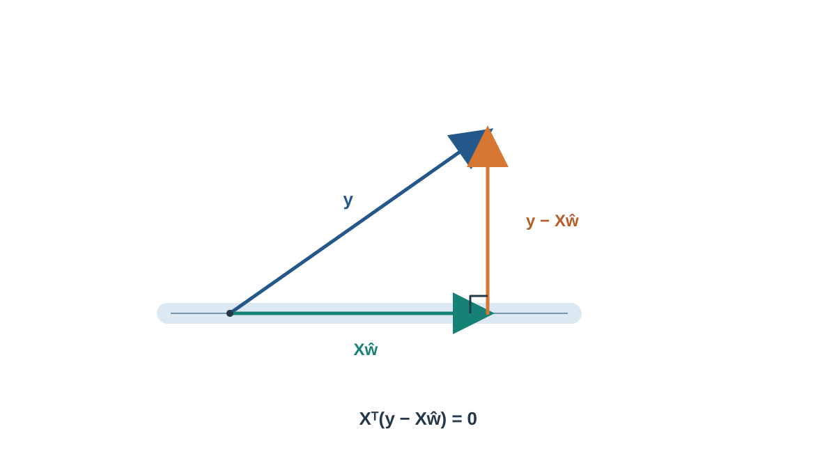
The algebra works, but it hides a picture worth seeing. Think of the columns of $X$ as vectors. Every linear combination of them — every possible prediction $Xw$ — lives in a subspace spanned by those columns. The observed target vector $y$ generally sits outside that subspace.

Least squares is then a geometry problem: find the point in the subspace closest to $y$. The closest point is the orthogonal projection of $y$ onto the subspace, and the residual $y - Xw$ is the perpendicular from $y$ down to it.

If the residual is perpendicular to the subspace, it must be perpendicular to every column of $X$. Write that as equations:

$X^\top (y - Xw) = 0$

Expand:

$X^\top y - X^\top X w = 0 \quad \Longrightarrow \quad X^\top X w = X^\top y$

The normal equations, from a different door. Same destination, no calculus required.

The geometry also tells you what the fit can and cannot do. The model can only produce predictions inside the subspace. The residual is the part of the data the model structurally cannot explain — not a failure of the solver, but a limit of the representation.

A Small Worked Example by Hand

Let's push numbers through the formulas. Take four points with one feature:

The design matrix includes the intercept column:

$X = \begin{bmatrix} 1 & 1 \\ 1 & 2 \\ 1 & 3 \\ 1 & 4 \end{bmatrix}, \qquad y = \begin{bmatrix} 2 \\ 4 \\ 5 \\ 9 \end{bmatrix}$

Compute the pieces of the normal equations. First $X^\top X$:

$X^\top X = \begin{bmatrix} 4 & 10 \\ 10 & 30 \end{bmatrix}$

Then $X^\top y$:

$X^\top y = \begin{bmatrix} 20 \\ 60 \end{bmatrix}$

Solve $X^\top X w = X^\top y$. The determinant of the Gram matrix is $4 \cdot 30 - 10 \cdot 10 = 20$, so:

$(X^\top X)^{-1} = \frac{1}{20}\begin{bmatrix} 30 & -10 \\ -10 & 4 \end{bmatrix}$

Multiply:

$\hat{w} = \frac{1}{20}\begin{bmatrix} 30 & -10 \\ -10 & 4 \end{bmatrix}\begin{bmatrix} 20 \\ 60 \end{bmatrix} = \frac{1}{20}\begin{bmatrix} 0 \\ 40 \end{bmatrix} = \begin{bmatrix} 0 \\ 2 \end{bmatrix}$

The intercept is $0$ and the slope is $2$: the fitted line is $\hat{y} = 2x$.

Now check the residuals:

The residuals sum to zero, and they are uncorrelated with the feature — the orthogonality property, visible in the numbers. The line also passes through the mean of $x$ (2.5) and the mean of $y$ (5), which is a general property of least-squares fits with an intercept.

You can confirm the result with a few lines of scikit-learn:

import numpy as np
from sklearn.linear_model import LinearRegression

X = np.array([[1], [2], [3], [4]])
y = np.array([2, 4, 5, 9])

model = LinearRegression().fit(X, y)
print(model.intercept_, model.coef_)  # 0.0 [2.]

The code verifies the derivation. It does not replace it — you now know which equation produced those numbers.

What the Coefficients and Residuals Are Telling You

Each coefficient is the expected change in the target for a one-unit change in that feature, holding the other features fixed. The slope of 2 above means each additional unit of $x$ adds 2 to the predicted $y$.

The intercept deserves care. It is the prediction when every feature is zero, which may be meaningless if zero lies outside the observed range. Here it is 0, but that is a fact about this dataset, not a universal rule.

Residuals are the model's leftover error, and their pattern matters more than their size. Well-behaved residuals look structureless — no curve, no funnel, no drift. A curved pattern suggests the linear form is wrong. A fan shape that widens with the feature suggests the error variance is not constant.

The derivation leans on a few assumptions: linearity in the parameters, independent observations, and roughly constant error variance. When those fail, the residuals show it. But note the boundary: the closed-form solution is still the least-squares answer even when assumptions are violated. The assumptions govern whether that answer is a good estimate, not whether it exists.

When the Closed Form Breaks Down

Three symptoms are worth recognizing.

Perfect collinearity. If one feature is an exact linear combination of others, the Gram matrix is singular, the inverse does not exist, and the solution is not unique. The model cannot distinguish the contributions of the redundant features.

Too many features. Forming and inverting $X^\top X$ costs roughly cubic time in the number of features. When that becomes the bottleneck, iterative methods earn their place.

Outliers and heavy-tailed noise. Squaring amplifies large residuals, so a few extreme points can pull the fit hard. The objective is doing exactly what it was defined to do — which is the problem.

The standard response to unstable or non-unique solutions is regularization, which adds a penalty that keeps the coefficients bounded and the solution unique. That is the natural next topic once the unregularized solution starts to wobble.

Where to Go Next

The derivation is now yours, not the library's. Two concrete moves will lock it in. First, re-derive the two-variable case on paper with your own numbers, then check the residuals sum to zero. Second, fit a small dataset and plot the residuals against the feature — if you see structure, you have found a violated assumption before any metric told you.

Once you can read a residual plot, the next question is what to do when the solution is unstable. That is where regularization picks up.