Build and Diagnose a Multiclass Classifier With Scikit-Learn

A model can score 94% accuracy and still be quietly failing one class. Here is how to see it.

You already know what multiclass classification is: each sample gets exactly one label from three or more classes. What you probably have not done yet is train one, look at the single accuracy number, feel satisfied, and then discover that the model has been confusing two classes the whole time. That gap between the headline number and the actual behavior is what this tutorial closes.

We will build the smallest runnable scikit-learn multiclass classification example, then spend most of our time reading the failure map instead of the score.

What You Need Before You Start

This is a practice tutorial, so the setup is short. You need Python with scikit-learn, NumPy, pandas, and matplotlib installed. If you have a working scientific Python environment, you are ready.

One thing worth stating plainly: scikit-learn classifiers handle multiclass natively. You do not need the sklearn.multiclass module to train a three-class model. That module exists for experimenting with decomposition strategies like one-vs-rest and one-vs-one, and we will touch it later as an optional comparison, not as a required step.

We will use the Iris dataset. It has 150 samples, four numeric features, and three balanced classes. It is small, deterministic, and boring in the best way: nothing about the data will distract you from the workflow.

By the end, you will have four things: a fitted classifier, a confusion matrix, per-class metrics, and one controlled comparison between two handling choices.

Load the Data and Split It Honestly

Start by loading the data and checking its shape. This is the first observable checkpoint.

from sklearn.datasets import load_iris
from sklearn.model_selection import train_test_split
import numpy as np

X, y = load_iris(return_X_y=True)

print("Features:", X.shape)
print("Labels:", y.shape)
print("Class counts:", np.bincount(y))

Expected output:

Features: (150, 4)
Labels: (150,)
Class counts: [50 50 50]

You have a 150-by-4 feature matrix and a target with 50 samples in each of three classes. Balanced, clean, and small enough to reason about by hand.

Now split it. Use stratify=y so each class keeps its proportion in both the training and test sets.

X_train, X_test, y_train, y_test = train_test_split(
    X, y, test_size=0.3, stratify=y, random_state=42
)

print("Train counts:", np.bincount(y_train))
print("Test counts:", np.bincount(y_test))

Expected output:

Train counts: [35 35 35]
Test counts: [15 15 15]

Stratification matters here for a specific reason. If you skip it, a random split can leave one class barely represented in the test set. Then your per-class metrics for that class are computed on a handful of samples, and they swing wildly between runs. You cannot diagnose a class you barely tested.

Tip: Set random_state on every split and every estimator in this tutorial. Reproducibility is not a formality. It is what lets you compare two runs and trust that the difference came from your change, not from a different random draw.

Fit a First Classifier and Read the Accuracy

Fit a small, interpretable baseline. Logistic regression is a good default because it is fast and its behavior is easy to reason about.

from sklearn.linear_model import LogisticRegression
from sklearn.metrics import accuracy_score

clf = LogisticRegression(max_iter=200, random_state=42)
clf.fit(X_train, y_train)

y_pred = clf.predict(X_test)
print("Accuracy:", accuracy_score(y_test, y_pred))

Expected output:

Accuracy: 0.9333333333333333

That is about 93%. On a 45-sample test set, that means roughly three mistakes. Feels good. Feels done.

It is not done. Accuracy is a single number, and a single number cannot tell you which classes failed or how they failed. A model that gets every setosa right and splits its mistakes between versicolor and virginica looks identical, in accuracy terms, to a model that makes three unrelated errors. Those are different problems with different fixes.

Even on a balanced dataset, a systematic confusion between two classes can hide behind a respectable accuracy score. The next section pulls that confusion into the open.

Build the Confusion Matrix and Read the Pattern

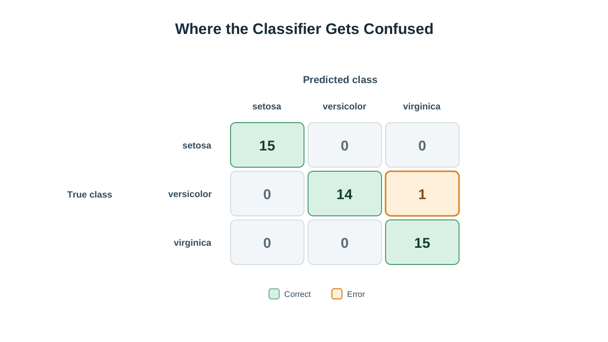
The confusion matrix turns one number into a class-by-class map of mistakes.

from sklearn.metrics import confusion_matrix

cm = confusion_matrix(y_test, y_pred)
print(cm)

Expected output:

[[15  0  0]
 [ 0 14  1]
 [ 0  0 15]]

Read it like this: rows are the true class, columns are the predicted class. The diagonal is correct predictions. Everything off the diagonal is a mistake.

Walk through it:

• True setosa (row 0): 15 predicted setosa, 0 predicted versicolor, 0 predicted virginica. Perfect.
• True versicolor (row 1): 14 predicted versicolor, 1 predicted virginica. One versicolor flower was called virginica.
• True virginica (row 2): 15 predicted virginica. Perfect.

The off-diagonal cell at row 1, column 2 is the real story. When the true class is versicolor, the model sometimes predicts virginica. That is a specific, diagnosable failure. It is not noise. It is a pattern, and patterns have causes: overlapping feature ranges, a decision boundary that sits in the wrong place, or a class that genuinely looks like another in the feature space.

Common mistake: Reading only the diagonal. The diagonal tells you what worked. The off-diagonal cells tell you what to fix. A large off-diagonal cell is a lead, not a rounding error.

A labeled heatmap makes the pattern scannable, but the numbers carry the lesson. If you want the visual, pass the matrix to matplotlib with class names on the axes. The interpretation does not change.

[[15, 0, 0],
 [0, 14, 1],
 [0, 0, 15]]

Go Beyond Accuracy With Per-Class Metrics

The confusion matrix shows you where the mistakes are. Per-class metrics tell you what kind of mistake each one is.

from sklearn.metrics import classification_report

print(classification_report(y_test, y_pred, target_names=["setosa", "versicolor", "virginica"]))

Expected output:

              precision    recall  f1-score   support

      setosa       1.00      1.00      1.00        15
  versicolor       1.00      0.93      0.97        15
   virginica       0.94      1.00      0.97        15

    accuracy                           0.93        45
   macro avg       0.98      0.98      0.98        45
weighted avg       0.98      0.98      0.98        45

Two terms to pin down before you read the table:

• Precision answers: when the model predicts this class, how often is it right?
• Recall answers: when this class is truly present, how often does the model find it?

Now read versicolor. Precision is 1.00, recall is 0.93. That means every versicolor prediction was correct, but one true versicolor was missed. The model is under-predicting versicolor. It is not over-calling it; it is failing to catch it.

Compare that to a hypothetical class with high recall and low precision. That class is over-predicted: the model finds it, but it also throws other classes into it. Same accuracy number, opposite problem, opposite fix.

The macro average treats every class equally. The weighted average follows class frequency. On balanced data like Iris, they nearly agree, and that agreement is itself a useful check: if macro and weighted diverge sharply, your classes are imbalanced and your accuracy number is hiding it.

Compare Two Handling Choices

One experiment is enough to see that handling choices change the confusion pattern, not just the score. Pick two.

Choice A: swap the classifier. Try a K-nearest neighbors model.

from sklearn.neighbors import KNeighborsClassifier

knn = KNeighborsClassifier(n_neighbors=5)
knn.fit(X_train, y_train)
knn_pred = knn.predict(X_test)

print(confusion_matrix(y_test, knn_pred))
print(classification_report(y_test, knn_pred, target_names=["setosa", "versicolor", "virginica"]))

KNN is sensitive to feature scale, so its confusion pattern may differ from logistic regression's. That difference is the point. You are not looking for a winner yet. You are looking for a different failure shape.

Choice B: keep the classifier, change a handling decision. Wrap the estimator in a pipeline that scales features first.

from sklearn.pipeline import Pipeline
from sklearn.preprocessing import StandardScaler

pipe = Pipeline([
    ("scale", StandardScaler()),
    ("clf", LogisticRegression(max_iter=200, random_state=42)),
])
pipe.fit(X_train, y_train)
pipe_pred = pipe.predict(X_test)

print(confusion_matrix(y_test, pipe_pred))

Scaling changes how the model weighs features, which can move the decision boundary and shift which samples land on the wrong side of it.

Note: scikit-learn classifiers already do multiclass internally, so OneVsRestClassifier and OneVsOneClassifier are for experimenting with decomposition strategies, not a required step. If you want to see how one-vs-one changes the pattern, wrap your estimator and compare. But keep the comparison to two options. The goal is to watch the confusion pattern shift, not to run a full model search.

Common Mistakes and How to Catch Them

These are the failure modes that make a multiclass workflow lie to you.

Fitting and evaluating on the same data. If you call fit and predict on the same X, your accuracy is inflated and your confusion matrix is too clean. The model has seen the answers. Always hold out a test set.

Forgetting stratify=y. Without it, a class can end up with two or three test samples. Per-class metrics on that few samples are unstable, and you will chase noise.

Reading only the diagonal. The diagonal is the scoreboard. The off-diagonal is the diagnosis. Train your eye on the cells that are not on the main diagonal.

Assuming high accuracy means all classes are handled well. This is the trap the whole article is built around. It gets worse with imbalanced classes, where a model can ignore a minority class entirely and still post a high accuracy.

Your Next Experiment

Here is the modification that makes the lesson stick. Deliberately imbalance the training data by dropping most samples of one class, then re-run the same workflow.

# Keep all setosa and versicolor, but only 5 virginica samples in training
virginica_idx = np.where(y_train == 2)[0]
keep_virginica = virginica_idx[:5]
mask = np.ones(len(y_train), dtype=bool)
mask[virginica_idx[5:]] = False

X_train_imb = X_train[mask]
y_train_imb = y_train[mask]

print("Imbalanced train counts:", np.bincount(y_train_imb))

clf_imb = LogisticRegression(max_iter=200, random_state=42)
clf_imb.fit(X_train_imb, y_train_imb)
y_pred_imb = clf_imb.predict(X_test)

print("Accuracy:", accuracy_score(y_test, y_pred_imb))
print(confusion_matrix(y_test, y_pred_imb))
print(classification_report(y_test, y_pred_imb, target_names=["setosa", "versicolor", "virginica"]))

Expected output:

Imbalanced train counts: [35 35  5]
Accuracy: 0.9333333333333333
[[15  0  0]
 [ 0 15  0]
 [ 0  3 12]]
              precision    recall  f1-score   support

      setosa       1.00      1.00      1.00        15
  versicolor       0.83      1.00      0.91        15
   virginica       1.00      0.80      0.89        15

    accuracy                           0.93        45
   macro avg       0.94      0.93      0.93        45
weighted avg       0.94      0.93      0.93        45

Look at what happened. Accuracy stayed at 93%—identical to the balanced baseline. But the confusion matrix tells a completely different story. Virginica recall dropped from 1.00 to 0.80: three virginica flowers were predicted as versicolor. The model has seen so few virginica examples that it now under-predicts that class, and the aggregate accuracy number never flinched.

That is the real-world case where accuracy is actively misleading. It is also why the workflow in this article matters more than any single model choice.

My rule for multiclass problems is simple: never trust a single accuracy number. Read the confusion matrix first. Check per-class precision and recall second. Only then decide whether the model is good enough. From here, the natural next step is tuning the model or handling class imbalance directly, and both of those decisions get easier once you can see which classes are actually failing.