Test KNN Neighbor Count and Feature Scaling With Scikit-Learn

Same data. Same code. Two accuracy scores that disagree, and nothing in the output explains why.

That gap is the whole point of this experiment. When you first meet K-nearest neighbors, n_neighbors and feature scaling look like two knobs you twist until the score improves. They are not. They are two separate mechanisms: one controls how many points vote, the other controls whether the vote is fair. Change them one at a time, and the output stops being a mystery and starts being evidence.

What This Experiment Is Actually Testing

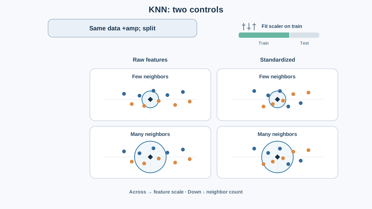
We are isolating two variables and holding everything else still.

• How many neighbors vote: the n_neighbors parameter.
• How distance is measured: the scale of your features.

Everything else stays fixed: one dataset, one train/test split with a fixed random_state, one metric (accuracy), one model family. If two things change between runs, you learn nothing about either.

You have already seen why KNN is a local, distance-based method and why scale affects distance. We will not re-derive that here. We are going to watch it happen.

Note: This is not a benchmark and not a hunt for the "best" k. It is a way to see cause and effect. The success criterion is simple: before you run each change, you should be able to predict which direction accuracy moves.

Set Up the Data and the Baseline Model

We need a dataset with features measured in different units, so scaling effects are visible. The Iris dataset works well: petal and sepal measurements are all in centimeters, but their ranges differ enough to matter.

from sklearn.datasets import load_iris
from sklearn.model_selection import train_test_split
from sklearn.neighbors import KNeighborsClassifier
from sklearn.metrics import accuracy_score

X, y = load_iris(return_X_y=True)

X_train, X_test, y_train, y_test = train_test_split(
    X, y, test_size=0.3, stratify=y, random_state=42
)

knn = KNeighborsClassifier(n_neighbors=5)
knn.fit(X_train, y_train)
preds = knn.predict(X_test)

baseline = accuracy_score(y_test, preds)
print(f"Baseline accuracy (k=5, unscaled): {baseline:.4f}")

Write that number down. It is the anchor for every comparison that follows.

Here is the part that surprises beginners: fit does almost nothing. KNN does not learn weights or coefficients. It stores the training data in an index structure so it can find neighbors quickly later. That is why training is cheap and prediction is the real cost. The model is not a formula. It is a memory.

Vary the Neighbor Count, Hold Everything Else Fixed

Now change only n_neighbors. Same split, same unscaled features, same metric.

for k in [1, 3, 5, 15, 50]:
    knn = KNeighborsClassifier(n_neighbors=k)
    knn.fit(X_train, y_train)
    acc = accuracy_score(y_test, knn.predict(X_test))
    print(f"k={k:>2}  accuracy={acc:.4f}")

You will get a small table of k versus accuracy. The point is not the winning row. The point is the shape of the change.

• Small k means each prediction follows a tiny local neighborhood. A single noisy point can flip the answer.
• Large k averages over a wide region. Noise gets suppressed, but the boundary between classes blurs.

This matches the standard framing: larger k suppresses noise but makes classification boundaries less distinct. You are trading sensitivity to local structure for smoothness.

Common mistake: k=1 often scores well on the training set and looks like the best choice. It is also the most fragile. A model that memorizes every training point has learned nothing that generalizes.

Add Feature Scaling and Compare Against the Baseline

Now introduce the second factor. Scaling changes how distance is computed.

Raw units distort distance. If one feature ranges into the thousands and another stays in single digits, the large-scale feature dominates the distance calculation — not because it is more useful, but because its numbers are bigger. The model silently weights features by their units.

from sklearn.preprocessing import StandardScaler

scaler = StandardScaler()
X_train_scaled = scaler.fit_transform(X_train)
X_test_scaled = scaler.transform(X_test)

for k in [1, 3, 5, 15, 50]:
    knn = KNeighborsClassifier(n_neighbors=k)
    knn.fit(X_train_scaled, y_train)
    acc = accuracy_score(y_test, knn.predict(X_test_scaled))
    print(f"k={k:>2}  scaled accuracy={acc:.4f}")

Warning: Fit the scaler on the training data only, then transform both train and test. Fitting on the full dataset leaks test information into training and inflates your results. The numbers will look better and mean less.

Compare this column against the unscaled table. The interesting result is usually the gap at small k, where distance dominates the prediction. Scaling does not add information. It removes an accidental, unit-driven bias in the distance metric.

Read the Decision Boundary, Not Just the Score

Accuracy is one number. The decision boundary is the shape of every decision the model makes. A decision boundary is the frontier between predicted classes — a visual summary of where the model changes its mind.

Plot the boundary for a two-feature slice of the data at a small k and a large k, unscaled versus scaled. What to look for:

• Small k: jagged, island-like regions. The model carves out tiny territories around individual points.
• Large k: smoother, more contiguous regions. The model generalizes across wider areas.
• After scaling: the boundary shifts. Regions that were distorted by unit imbalance get corrected.

Here is the trap: accuracy can stay flat while the boundary changes shape. Two models with identical scores can behave completely differently on new data. The score hides that difference. The boundary reveals it.

Keep the plot small and readable. You are looking for a pattern, not a polished figure.

Common Mistakes and How to Spot Them

These are the failure modes that make this experiment lie to you.

Mistake	Signal
Scaling before the split	Results look better than they are and will not reproduce on new data
Changing two factors at once	You cannot attribute the change to either one
Judging by training accuracy	k=1 scores near-perfect on training and means nothing
Tuning k on the test set	The test set quietly becomes a training set
Fragile comparisons	Results shift when you change random_state

That last one deserves attention. If your conclusion flips when you change the random seed, the comparison was never stable. A real effect survives a different split.

One More Experiment: Change the Distance Metric

You have changed how many points vote and how distance is measured through scale. There is a third lever: the shape of distance itself.

Swap Euclidean distance for Manhattan distance and re-run the same k sweep.

for k in [1, 3, 5, 15, 50]:
    knn = KNeighborsClassifier(n_neighbors=k, metric="manhattan")
    knn.fit(X_train_scaled, y_train)
    acc = accuracy_score(y_test, knn.predict(X_test_scaled))
    print(f"k={k:>2}  manhattan accuracy={acc:.4f}")

Before you run it, predict the direction of change. Write it down. Then run it and compare.

The metric defines what "near" means, so changing it changes which points vote. That is the same mechanism as scaling, applied to the shape of distance rather than its units. Euclidean distance measures straight-line distance. Manhattan distance measures distance along axes. Different geometry, different neighbors, different predictions.

The Rule That Outlasts This Experiment

In KNN, k controls how wide the vote is, and scaling controls whether the vote is fair. Everything else in this article is a consequence of those two facts.

The habit worth keeping is the method, not the numbers: change one factor, write down your prediction, run it, compare against the baseline. That loop turns any model from a black box into something you can reason about.

Your next step is to wrap the scaler and classifier into a single Pipeline. That enforces the correct order — fit the scaler on training data, then transform — by construction instead of by memory. Once the order is guaranteed, you can focus on the experiment instead of the plumbing.