
Fit and Inspect Logistic Regression With Scikit-Learn
You call predict(), and you get back a tidy row of zeros and ones. Clean. Decisive. And completely silent about the thing you actually wanted to see: the…

Key topics
You call predict(), and you get back a tidy row of zeros and ones. Clean. Decisive. And completely silent about the thing you actually wanted to see: the probability.
That silence is where beginners get stuck. The model didn't throw away the probability — it computed one, then applied a rule you never wrote. In this tutorial, you'll fit a logistic-regression classifier, pull the probabilities out into the open, watch them turn into labels, and then move the decision line yourself to see what changes.
If you've read the concept piece on how a linear score becomes a probability through the logistic function, this is the practice half. We won't re-derive the sigmoid. We'll make it run.
What You Need Before You Fit Anything
You need Python 3.8 or newer, plus scikit-learn, NumPy, and pandas. Scikit-learn depends on NumPy and SciPy, so installing it pulls those in. If you're starting fresh:
pip install scikit-learn pandas
We'll use a small built-in dataset so the whole experiment runs in seconds. The point is the model, not the data wrangling — I'd rather you spend your attention on probabilities than on CSV parsing.
Here's the success criterion. By the end of this article you will have:
- a fitted classifier,
- a table showing true labels next to predicted probabilities,
- and two different confusion matrices produced by two different thresholds.
That's it. Three artifacts, all yours.
Note: A quick bridge from the concept article. Logistic regression computes a linear score, pushes it through the logistic function, and gets a number between 0 and 1. That number is a probability. Everything below is about what happens after that number exists.
Split the Data and Fit the Classifier
Load the data and split it. Fix random_state so your output matches mine.
from sklearn.datasets import load_breast_cancer
from sklearn.model_selection import train_test_split
from sklearn.linear_model import LogisticRegression

X, y = load_breast_cancer(return_X_y=True)

X_train, X_test, y_train, y_test = train_test_split(
    X, y, test_size=0.25, random_state=42, stratify=y
)

model = LogisticRegression(max_iter=1000)
model.fit(X_train, y_train)
Two things worth naming.
First, fit() is where learning happens. The model searches for coefficients that minimize log loss — the penalty for assigning low probability to the correct class. This is not least squares. Linear regression minimizes squared error; logistic regression minimizes a different objective because its output is a probability, not a number on a line.
Second, scikit-learn applies L2 regularization by default. That surprises people coming from statistics, where unregularized logistic regression is the norm. In machine learning workflows, regularization is standard because it improves numerical stability and helps generalization. You can control its strength with the C parameter, but don't tune it yet. One thing at a time.
Now sanity-check the fit:
print(model.coef_.shape)       # (1, 30)
print(model.intercept_.shape)  # (1,)
One coefficient per feature, one intercept. If those shapes look wrong, something upstream is off.
Warning: You may see a
ConvergenceWarningaboutmax_iter. It means the optimizer hit its iteration limit before settling. It does not mean the model is broken. Raisingmax_iteris the first fix, and it's usually the only one you need.
Knowledge check
Check your understanding
Answer this question before you continue.
Read the Probabilities, Not Just the Labels
Here's the part that predict() hides. predict_proba() returns one column per class. Column 0 is P(class = 0); column 1 is P(class = 1). You almost always want the second column:
proba = model.predict_proba(X_test)[:, 1]
preds = model.predict(X_test)
Now build the table you'll keep. This is the artifact that makes the model legible:
import pandas as pd

inspect = pd.DataFrame({
    "true": y_test,
    "proba": proba.round(3),
    "pred": preds,
})
print(inspect.head(10))
You'll see rows where the true label is 1, the probability is 0.51, and the prediction is 1 — and rows where the probability is 0.99 and the prediction is also 1. Same label. Wildly different confidence.
That gap is the whole story. predict() is just predict_proba() plus a 0.5 cutoff. The label is a decision layered on top of the probability, not a separate model output. When you see 0.51 and 0.99 collapse into the same "1," you're watching the threshold do its work — and quietly throwing away information.
Common mistake: Reading
predict_probaoutput as a calibrated probability of being correct. It isn't. It's a model score. A 0.9 doesn't guarantee a 90% hit rate. Calibration is a separate question with its own tools, and we're not touching it here.
Knowledge check
Check your understanding
Answer this question before you continue.
Turn Probabilities Into Decisions With a Threshold
The default 0.5 is a convention, not a law. It's the right default only when both kinds of error cost roughly the same. Often they don't.
Converting probabilities to labels by hand takes one line:
threshold = 0.5
manual_preds = (proba >= threshold).astype(int)
Three tokens of code, full control. Compare manual_preds to preds and they'll match — that's the default threshold, written out loud.
Why would you ever move it? Consider two scenarios with the same model:
| Scenario | Worse mistake | Sensible threshold |
|---|---|---|
| Spam filter | Marking real mail as spam | Higher (be conservative) |
| Disease screening | Missing a sick patient | Lower (catch more) |
Same probabilities. Different costs. Different decisions. The model doesn't know which world it's in — you do.
This connects directly to precision and recall. Lower the threshold and you flag more positives: recall rises, precision falls. Raise it and the reverse happens. The threshold is a business decision expressed in code.
Knowledge check
Check your understanding
Answer this question before you continue.
Run the Threshold Experiment
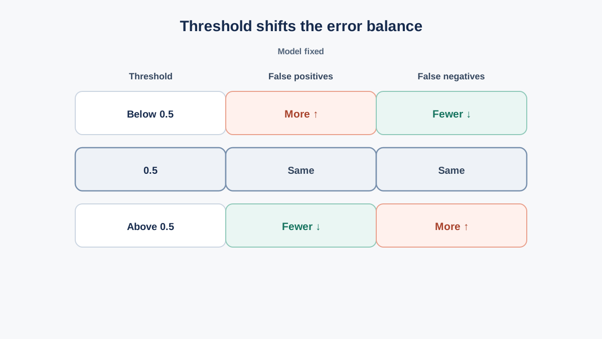
Now the controlled experiment. Hold the model fixed. Change only the threshold. That's what makes it an experiment instead of a fishing trip.
Before you run it, predict the outcome. Lowering the threshold should raise recall and lower precision. Raising it should do the reverse. State that prediction, then check it against the output.
from sklearn.metrics import confusion_matrix, precision_score, recall_score

for t in [0.3, 0.5, 0.7]:
    labels = (proba >= t).astype(int)
    cm = confusion_matrix(y_test, labels)
    print(f"threshold={t}")
    print(cm)
    print(f"  precision={precision_score(y_test, labels):.3f}")
    print(f"  recall={recall_score(y_test, labels):.3f}")
The confusion matrix is the clearest view of what changed. Read it as counts of false positives and false negatives. At 0.3 you'll see more false positives and fewer false negatives. At 0.7, the reverse. The precision and recall numbers just summarize what the matrix already shows.
Debugging signal: If nothing changes across thresholds, your probabilities are probably clustered near 0 and 1. That's worth noticing on its own — it means the model is very confident, and the threshold has little room to maneuver.
Knowledge check
Check your understanding
Answer this question before you continue.
Pick a Threshold You Can Defend
Start from the cost of each error type, not from a target accuracy number. Ask which mistake is worse, and by how much. That ratio tells you which direction to move.
Then use the validation set to choose the threshold, and report on the test set once. If you tune the threshold on the test set, you've quietly turned it into training data — the same trap the train/validation/test article warns about, just wearing a different hat.
Two boundaries worth respecting:
- Threshold tuning cannot fix a model whose probabilities are uninformative. If the ranking is bad, no cutoff saves it. You're just choosing which way to be wrong.
- If the downstream system consumes the probability directly — a ranking, a risk score, a queue — you may never need a hard label at all. Sometimes the best threshold is no threshold.
Where to Take This Next
One modification to try right now: add a second feature, or swap in your own CSV, and rerun the same threshold loop. Watch how the probability distribution shifts and whether the threshold still has room to move.
The natural next step is wrapping the scaler and classifier into a Pipeline, so the same preprocessing is applied consistently at fit and predict time. That's where this stops being a script and starts being a reusable component.
But the durable idea is simpler. The model produces a ranking. The threshold turns that ranking into a decision. And the decision belongs to you — not to the 0.5 that scikit-learn quietly picked on your behalf.
Knowledge check
Final check
Finish the article by checking the ideas you just learned.
References
Build stronger machine learning foundations
Use structured resources to connect theory, scikit-learn workflows, and evaluation practice.


