
KNN Regression as Local Averaging: Neighborhood Size, Bias, and Variance
Fit KNN regression with k=1 and the prediction curve threads through every training point. Set k=50 and the same curve flattens toward a horizontal line.…

Key topics
Fit KNN regression with k=1 and the prediction curve threads through every training point. Set k=50 and the same curve flattens toward a horizontal line. The natural conclusion is that small k is accurate and large k is smooth — that k is an accuracy dial you turn toward "better."
That conclusion is wrong, and it produces bad models. k is not an accuracy dial. It is a bandwidth: the width of a window you slide across the input space, averaging whatever responses fall inside. Widen the window and you smooth away noise, but you also average across regions where the true relationship has already moved. Narrow it and you track the data exactly, including the parts that are pure noise.
This article derives the prediction as a neighborhood average, works a small example by hand, and then reasons carefully about how the window width trades smoothing bias against local variance. The goal is a mechanism you can reason from — not a magic number to copy.
What the Prediction Actually Computes
Start with notation, because every later claim depends on these symbols meaning something concrete.
You have a training set of pairs:
Each is a feature vector, each is a real-valued response. You want to predict at a query point — a point that may or may not be in the training set.
First you need a notion of "near." The default is Euclidean distance:
Then you sort the training points by that distance and take the closest. Call that set — the neighborhood of .
The prediction is the plain average of their responses:
That is the entire estimator. Read it once more, because the simplicity hides the design: the weights are for points inside the neighborhood and for points outside. It is a local averaging estimator with a hard-edged, uniform kernel. Every neighbor counts equally; every non-neighbor counts not at all.
Contrast this with a global linear fit. Linear regression learns one rule — a single set of coefficients — and applies it everywhere. KNN learns nothing in advance. It constructs a fresh rule for every query point, using only the data that happens to sit nearby. One rule for all of space versus a new rule per question.
Two structural choices hide inside the definition, and both matter later:
- The metric. Euclidean is the default, not a law. Change the metric and you change which points count as neighbors.
- The weighting scheme. Uniform weights are the simplest choice. Distance-weighted variants exist, but the uniform version is what makes the bias-variance analysis clean.
Knowledge check
Check your understanding
Answer this question before you continue.
A Worked Example You Can Check by Hand
Small numbers make the mechanism visible. Take a one-dimensional dataset:
| 0 | 1 | 2 | 3 | 4 | 5 | |
|---|---|---|---|---|---|---|
| 1 | 3 | 2 | 5 | 4 | 6 |
Query at . Compute distances:
| 2 | 3 | 1 | 4 | 0 | 5 | |
|---|---|---|---|---|---|---|
| 0.6 | 0.4 | 1.6 | 1.4 | 2.6 | 2.4 | |
| 2 | 5 | 3 | 4 | 1 | 6 |
Sorted by distance: (0.4), (0.6), (1.4), (1.6), (2.4), (2.6).
Now compute the prediction at three values of :
- : nearest neighbor is , so .
- : neighbors are , so .
- : neighbors are , so .
Same query point, three different answers. Nothing about the data changed — only the window width.
Two boundary cases are worth naming. At , the prediction equals a single training response, so the fitted curve passes exactly through every training point. At , the neighborhood is the entire dataset and the prediction collapses to the global mean of — here, . The estimator loses all locality. Between those extremes, slides the prediction from "trust one noisy observation" to "trust nothing but the overall average."
Here is the same arithmetic in code, purely to confirm the hand calculation:
import numpy as np

x = np.array([0, 1, 2, 3, 4, 5], dtype=float)
y = np.array([1, 3, 2, 5, 4, 6], dtype=float)
x0 = 2.6

order = np.argsort(np.abs(x - x0))
for k in (1, 3, 5):
    print(k, y[order[:k]].mean())
Run it and you get 5.0, 3.666..., 4.0. The derivation and the output agree, which is the only reason to write the code at all.
Knowledge check
Check your understanding
Answer this question before you continue.
Where the Average Comes From
The estimator looks arbitrary until you derive it from the quantity you actually want.
Regression, stated formally, is the problem of estimating the conditional mean:
If you knew exactly, you would never need KNN. You do not know it, so you estimate it from samples. The natural estimate of a conditional mean is a sample mean — but only of samples that are conditioned on being near . That is precisely what the neighborhood average does:
The approximation sign is doing real work. It leans on two assumptions:
- Smoothness. The true regression function is roughly constant inside the neighborhood, so for every neighbor.
- Locality. The neighborhood is small enough that its points are genuinely informative about , not about some distant region.
Write each response as signal plus noise, , with noise mean zero and variance . Substitute into the estimator:
The first term is the average of the true function over the neighborhood. The second is the average of the noise. Now take expectations over the noise. The noise term averages to zero, so the bias is the gap between that first term and the truth:
This is the average distance between at the neighbors and at the query point. If is flat across the neighborhood, the bias is zero. If is climbing or falling, the neighbors sit above or below on average, and the bias is nonzero. The smoothness assumption is what keeps this term small.
The variance comes from the noise term. Under the simplifying assumption that the noise values are independent across neighbors:
Average independent noise draws and the variance of the average shrinks by a factor of . More neighbors, less jitter.
Note: That term is a clean idealization, not a promise. It is conditional on the neighbor locations staying fixed and the noise being independent and equally variable across neighbors. Real neighbors are not independent draws — nearby points often share unmeasured structure, so their noise is correlated. When noise is positively correlated across neighbors, the variance falls more slowly than . Treat the formula as the direction of the effect, not a precise prediction.
Knowledge check
Check your understanding
Answer this question before you continue.
Why k Is a Bandwidth, Not an Accuracy Dial
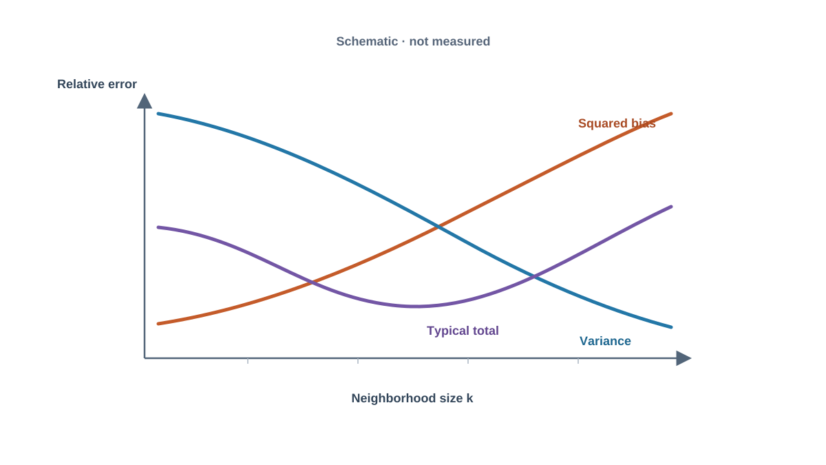
Now the two terms can be read against each other, and the tradeoff appears as a consequence rather than a slogan.
Small . The neighborhood hugs , so and the bias term is tiny. But the prediction rides on very few noisy responses, and is large. Resample the training set and the prediction at jumps around. Low bias, high variance.
Large . Many responses get averaged, so the variance term shrinks. But the neighborhood now spans regions where has already moved, so the bias term tends to grow. The prediction is stable and consistently wrong in curved regions. Low variance, high bias.
The two movements usually run in opposite directions:
- Bias tends to rise with — a wider window averages over more of 's variation.
- Variance falls roughly as — more terms in the average means less jitter.
Expected squared error at is the sum of a squared bias term, a variance term, and the irreducible noise :
One term tends to climb as grows. One term falls. Their sum often traces a U-shaped curve, and the minimum of that curve is the neighborhood size that balances the two for this particular problem.
Here is where the tidy story needs a boundary. The assumptions we listed — local smoothness and independent, mean-zero noise — do not guarantee that the bias term increases monotonically as you add neighbors. Adding a neighbor can move the average of closer to , farther from it, or across it, depending on the shape of , the geometry of the neighborhood, and the order in which points enter. What the assumptions support is a tendency, not a theorem: wider windows smooth more, and smoothing more usually costs bias in curved regions. The U-shape is a common and useful pattern, not a consequence the current derivation proves pointwise.
Common mistake: Treating the U-shape as a universal law of all models. It is a property of this estimator under these assumptions, and even here it is a tendency rather than a guarantee. The bias-variance tradeoff is well documented for KNN and kernel regression, but it is not guaranteed for every model class, and it should not be assumed without checking.
Knowledge check
Check your understanding
Answer this question before you continue.
What Breaks the Clean Picture
The derivation above is tidy because it assumes a lot. Each assumption is a place where the analysis stops applying.
Feature scaling. Distances are computed across all features at once. If one feature ranges over thousands and another over single digits, the large-range feature dominates the distance calculation entirely. The "neighborhood" becomes a slice defined by one variable, and the local average is no longer local in any meaningful sense. Standardize features before trusting any of this.
The curse of dimensionality. In high dimensions, the nearest neighbors are barely closer to than randomly chosen points. When everything is roughly equidistant, "near" stops meaning near, the smoothness assumption fails, and the bias argument collapses. This is the single biggest reason KNN struggles as feature count grows.
Non-uniform data density. The same produces a wide neighborhood in sparse regions and a narrow one in dense regions. So the effective bandwidth varies across the input space even though is fixed. In sparse regions you get high bias; in dense regions you get high variance. One number, two different behaviors.
Boundary effects. Near the edges of the data, neighborhoods are one-sided — all neighbors lie to one side of . The average is pulled inward, and predictions at the boundary are systematically biased toward the interior.
Ties and metric choice. Duplicate distances create ambiguity about which points enter the neighborhood. And switching from Euclidean to Manhattan distance changes the neighborhood itself, which changes every downstream number.
From Estimator Analysis to a Practical Choice
The theory tells you the shape of the tradeoff. It does not hand you a number.
The right depends on the sample size , the noise level , the smoothness of , and the local density of your data. Change any of those and the optimal window width moves. That is why there is no universal best — any single recommended value is a heuristic, not a result. The same that underfits one dataset overfits another.
The practical procedure is straightforward: choose by cross-validated error under a fixed evaluation setup, then read the resulting curve as an empirical picture of the bias-variance tradeoff you just derived. A validation curve that dips and rises is the U-shape showing up in your actual data.
One caution before you read that curve too literally. The result above held the neighbor locations fixed and varied only the noise. Cross-validation does something different: it refits the model on different training subsets, so the neighbor locations themselves change, and the variance you observe includes that resampling effect. The empirical curve and the clean formula are related, not identical. Use the formula for intuition and the curve for decisions.
My rule is to start moderate, inspect the validation curve, and treat as a smoothing parameter I can justify rather than a default I inherited. If the curve is flat across a range of , the problem is insensitive to the choice and you can pick for convenience. If it has a sharp minimum, the choice matters and you should report how you made it.
This is estimator-level reasoning, not a benchmarking exercise. The goal here is to understand the mechanism — why the average behaves the way it does — not to produce a leaderboard number. Tuning KNN for a specific classification task is a separate workflow with its own evaluation discipline.
The next move is concrete. Take a small one-dimensional dataset, fit KNN regression at , and plot all three prediction curves over the same scatter. Watch the curve thread through every point, watch the curve flatten, and watch the middle one trade a little of each. The tradeoff stops being a slogan the moment you see it as a shape — and the number you eventually choose will be one you earned through validation, not one you copied from a tutorial.
Knowledge check
Final check
Finish the article by checking the ideas you just learned.
References
Build stronger machine learning foundations
Use structured resources to connect theory, scikit-learn workflows, and evaluation practice.


