When Is Least Squares Unbiased? Assumptions Behind OLS Guarantees

A coefficient can be unbiased on average and still be wrong in your one dataset. Worse, it can be unbiased and still predict badly, and unbiased and still carry no causal meaning. Those are three different failures, and they come from three different assumptions.

You can already fit a least-squares line. You can read residuals, compute an R², and print a coefficient table. Somewhere along the way you absorbed the sentence "OLS is unbiased" and filed it as a property of your fitted model. It is not. It is a property of a procedure under a contract, and if you cannot name the clauses of that contract, you cannot tell when you have voided it.

This article fixes the target of the guarantee, states the classical setup, derives where unbiasedness comes from, derives where the variance result comes from, and then shows why neither property survives a misspecified model or licenses a causal claim.

What "Unbiased" Actually Claims

The OLS estimate is a random variable. That sentence is the whole game, and it is the one most learners skip.

Imagine the data-generating process as a machine that emits a fresh dataset of size n every time you press a button. You press it, fit OLS, and get a coefficient vector. You press it again and get a slightly different one. Press it a thousand times and you have a thousand coefficient vectors — a sampling distribution.

Unbiasedness is a statement about the mean of that distribution:

$\mathbb{E}[\hat{\beta}] = \beta$

The average of the estimates across repeated samples equals the true parameter. That is all it says.

It does not say your estimate is close to β. It does not say your estimate is correct. It says that if you could run the experiment forever, the errors would cancel. In any single sample — the only sample you will ever have — an unbiased estimator can be far off.

The error of an estimator decomposes into two pieces:

$\mathbb{E}[(\hat{\beta} - \beta)^2] = \underbrace{(\mathbb{E}[\hat{\beta}] - \beta)^2}_{\text{bias}^2} + \underbrace{\mathbb{E}[(\hat{\beta} - \mathbb{E}[\hat{\beta}])^2]}_{\text{variance}}$

Unbiasedness zeroes the first term. It says nothing about the second. A procedure can be perfectly unbiased and so noisy that any given estimate is useless. Hold that frame: the rest of this article is about which assumptions zero the bias term, which assumptions control the variance term, and why neither term answers the prediction or causal question.

The Setup and Notation

Write the classical linear model as

$y = X\beta + \varepsilon$

where $y$ is an $n \times 1$ vector of outcomes, $X$ is an $n \times p$ design matrix whose rows are observations and columns are regressors, $\beta$ is the $p \times 1$ vector of true parameters, and $\varepsilon$ is the $n \times 1$ vector of errors.

The OLS estimator is

$\hat{\beta} = (X^\top X)^{-1} X^\top y$

which requires $X^\top X$ to be invertible — equivalently, $X$ must have full column rank. This is the normal-equation solution you already derived; I will not re-derive it here. What matters now is the distinction between two objects that look similar and behave nothing alike:

• $\varepsilon = y - X\beta$ is the true error. You never observe it. It is a property of the data-generating process.
• $e = y - X\hat{\beta}$ is the residual. You compute it every time you fit. It is a property of your sample and your estimate.

Conflating them is the source of most confusion about OLS assumptions. The assumptions below are about $\varepsilon$ and $X$. They are not about $y$ alone, and they are not about $e$.

Assumptions That Buy Unbiasedness

Substitute the model into the estimator:

$\hat{\beta} = (X^\top X)^{-1} X^\top (X\beta + \varepsilon) = \beta + (X^\top X)^{-1} X^\top \varepsilon$

Take the conditional expectation given $X$:

$\mathbb{E}[\hat{\beta} \mid X] = \beta + (X^\top X)^{-1} X^\top \mathbb{E}[\varepsilon \mid X]$

The second term vanishes whenever $\mathbb{E}[\varepsilon \mid X] = 0$, which gives $\mathbb{E}[\hat{\beta} \mid X] = \beta$. This is the zero conditional mean assumption, and it is the standard sufficient condition for conditional unbiasedness.

Read the algebra carefully, because the direction of the implication matters. Zero conditional mean is enough to guarantee unbiasedness. It is not the only way the second term can vanish — a nonzero conditional error mean could in principle be annihilated by the particular matrix weighting $(X^\top X)^{-1} X^\top$. But that weaker moment condition is not something you can verify or reason about in practice. Zero conditional mean is the condition you actually check, and it is the one the rest of this article assumes.

Operationally, the assumption says that knowing $X$ does not systematically shift the average error. It does not say the errors are independent of $X$, and it does not say the error distribution is the same at every value of $X$. The conditional mean is zero; the conditional variance can still move with $X$, as the next section shows.

In practice the assumption fails whenever:

• A relevant variable is omitted and correlated with an included regressor.
• A regressor is measured with systematic error.
• The outcome and a regressor are jointly determined, so the regressor absorbs part of the error.

A worked example

Suppose the true process is $y = 2 + 3x_1 + 4x_2 + \varepsilon$ with $\mathbb{E}[\varepsilon \mid x_1, x_2] = 0$. You fit only $x_1$:

$y = \alpha + \beta_1 x_1 + u, \quad u = 4x_2 + \varepsilon$

The composite error $u$ now contains $x_2$. If $x_2$ is correlated with $x_1$ — say $\text{Cov}(x_1, x_2) = c \neq 0$ — then $\mathbb{E}[u \mid x_1] \neq 0$, and the omitted-variable formula gives

$\mathbb{E}[\hat{\beta}_1] = 3 + 4 \cdot \frac{\text{Cov}(x_1, x_2)}{\text{Var}(x_1)}$

With $c = 0.5$ and $\text{Var}(x_1) = 1$, the expected estimate is $3 + 2 = 5$. Not close. Not noisy. Systematically wrong, and no sample size fixes it — the bias term does not shrink as $n$ grows. More data sharpens your estimate of the wrong number.

Where the Variance Result Comes From

Unbiasedness is half the story. The other half is how much $\hat{\beta}$ moves across samples. Under spherical errors — constant variance and zero covariance across observations — the sampling variance is

$\text{Var}(\hat{\beta} \mid X) = \sigma^2 (X^\top X)^{-1}$

Two assumptions enter here and only here:

• Homoscedasticity: $\text{Var}(\varepsilon_i \mid X) = \sigma^2$ for all $i$. Constant error variance.
• No autocorrelation: $\text{Cov}(\varepsilon_i, \varepsilon_j \mid X) = 0$ for $i \neq j$. Errors are uncorrelated across observations.

Neither is required for unbiasedness. This is the split that matters: violate homoscedasticity and $\hat{\beta}$ is still unbiased, but the usual standard errors are wrong. Confidence intervals get the wrong width. t-tests get the wrong p-values. You will report a precise-looking result that is not precise, or miss a real effect because the interval is too wide.

The $(X^\top X)^{-1}$ term carries a second lesson. When columns of $X$ are nearly linearly dependent, $X^\top X$ approaches singularity and its inverse inflates. Coefficients become highly sensitive to small perturbations in $y$. This is multicollinearity: variance inflation without bias. The estimate is still centered on β; it just wanders further from it in any given sample.

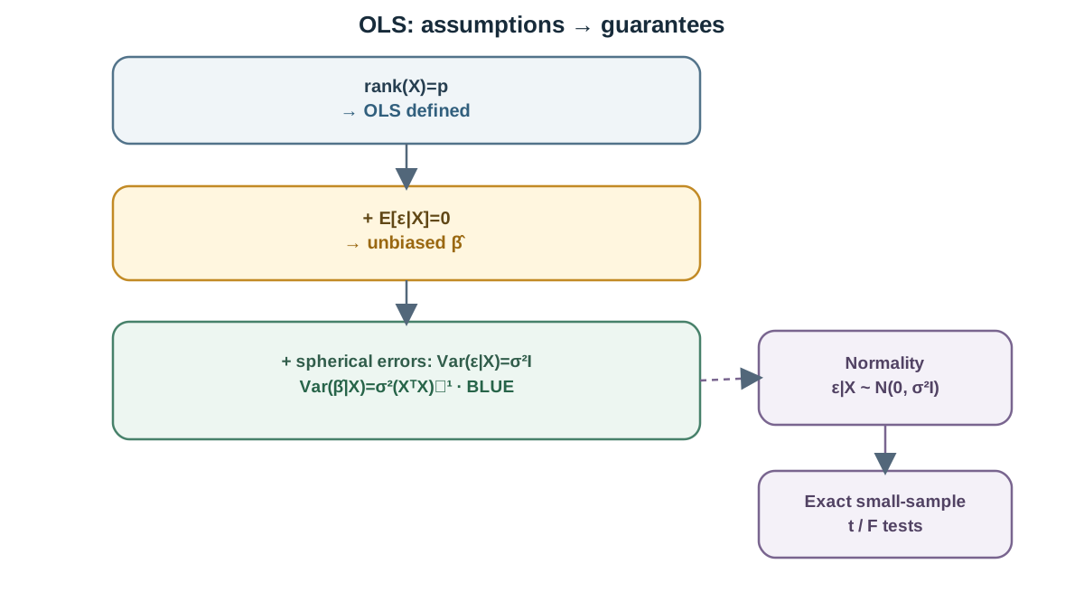
One more boundary: normality is not required for unbiasedness or for the Gauss-Markov variance result. It is required for exact small-sample t and F distributions. In large samples, the central limit theorem makes those tests approximately valid without it.

Gauss-Markov: What BLUE Does and Does Not Promise

The Gauss-Markov theorem states that under the classical assumptions — linearity in parameters, full rank, $\mathbb{E}[\varepsilon \mid X] = 0$, homoscedasticity, and no autocorrelation — OLS is the Best Linear Unbiased Estimator.

Unpack each word, because the theorem is narrower than its reputation:

• Linear: restricted to estimators that are linear functions of $y$.
• Unbiased: restricted to estimators with zero bias.
• Best: minimum variance within that restricted class.

"Best" is a within-class claim. It does not say OLS beats every estimator. It says OLS beats every linear unbiased estimator. Step outside the class and the guarantee evaporates.

Ridge regression is the concrete counterexample. By accepting a small amount of bias, ridge can achieve lower mean squared error than OLS — the bias term grows, but the variance term shrinks faster. That trade is exactly the bias-variance decomposition from the first section, made operational. BLUE is a reason to trust OLS when the assumptions hold. It is not a reason to stop checking them.

Unbiased Coefficients, Bad Predictions

Estimating β and predicting $y$ at new values of $X$ are different problems. Unbiasedness answers the first. It says nothing about the second.

Expected squared prediction error at a new point $x_0$ decomposes into irreducible noise, squared bias, and variance:

$\mathbb{E}[(y_0 - \hat{y}_0)^2] = \sigma^2 + \text{Bias}^2 + \text{Var}(\hat{y}_0)$

An unbiased estimator contributes zero to the middle term and can still contribute heavily to the last one. High-variance coefficients produce high-variance predictions. The model is right on average and unstable in practice.

Two failure modes deserve names:

Extrapolation. A model unbiased on the training distribution can be badly wrong outside the observed range of $X$. The linear form is an assumption, not a fact, and nothing in the data constrains behavior beyond the range you observed.

Large irreducible noise. Even a correctly specified conditional mean gives poor point predictions when $\sigma^2$ is large. The signal is thin; the noise dominates.

The practical signal is simple: compare training error to held-out error, and inspect where the model is being asked to predict relative to the data it saw. If the new $X$ values sit outside the training range, treat the prediction as an extrapolation, not an estimate.

Unbiased Coefficients, Wrong Causal Story

Here is the trap that catches experienced practitioners. Unbiasedness is defined relative to the model you wrote down. It says nothing about whether that model matches the causal structure of the world.

$\mathbb{E}[\varepsilon \mid X] = 0$ can hold perfectly for a purely predictive specification while the coefficient has no causal interpretation. The regression is doing its job — estimating a conditional mean — and you are asking it a question it was never built to answer.

The threats that survive a clean regression:

• Confounding: an unmeasured variable drives both $X$ and $y$.
• Simultaneity: $X$ and $y$ determine each other.
• Selection: the sample was chosen in a way correlated with the outcome.
• Measurement error in regressors: attenuates coefficients in ways that mimic real effects.

The same coefficient can be unbiased for a descriptive conditional mean and meaningless as an effect estimate. Causal claims require a design or identification argument — randomization, an instrument, a discontinuity, a defensible set of controls — that regression mechanics cannot supply. The math will not warn you. It will hand you a tight confidence interval around a number that means nothing.

Diagnosing Violations in Practice

Turn each assumption into a check you can run.

Assumption	What it protects	How to check	What to do when it fails
$\mathbb{E}[\varepsilon \mid X] = 0$	Unbiasedness	Residuals vs. each regressor; domain reasoning about omitted variables	Add controls, change design, or abandon causal claims
Homoscedasticity	Standard errors	Residual variance vs. fitted values	Heteroscedasticity-consistent standard errors
No autocorrelation	Standard errors	Residual correlation for time-ordered or grouped data	Cluster-robust or Newey-West standard errors
Full rank / low collinearity	Coefficient stability	Condition number or variance inflation factors	Drop, combine, or regularize regressors
Normality (optional)	Exact small-sample tests	Residual QQ plot	Rely on asymptotic tests, or bootstrap

The decision rule splits by goal:

• If the goal is inference, fix the standard errors first, then interrogate the design. A heteroscedasticity-robust or cluster-robust standard error costs nothing and removes a whole class of false confidence.
• If the goal is prediction, validate on held-out data and consider regularized or more flexible models. Unbiasedness is not the metric you care about; out-of-sample error is.

Common mistake: Treating a high R² or a significant p-value as evidence that the model is correct. Both can survive severe assumption violations. Neither is a substitute for checking $\mathbb{E}[\varepsilon \mid X] = 0$.

The One Rule to Carry Forward

Unbiasedness is a conditional promise about the average of an estimator across repeated samples. It is bought by the zero-conditional-mean assumption and paired with a variance result that depends on spherical errors. Neither property survives a misspecified model. Neither licenses a causal claim. Neither guarantees a good prediction.

The next move is concrete. Take a model you have already fit. Plot the residuals against each regressor, one at a time. Look for structure — curvature, fanning, clusters. Then ask the question that actually determines whether you can trust the coefficient: is it plausible that $\mathbb{E}[\varepsilon \mid X] = 0$ here? If you cannot answer yes with a reason, you have a descriptive fit, not an estimate you can build a decision on.