Least-Squares Residuals as Projections: Why Orthogonality Appears

You fit a line, plot the residuals, and they look like a clean cloud. No funnel, no curve, no obvious outlier. It is tempting to read that plot as a certificate: the model is correct. It is not. The cleanliness you are seeing is partly a geometric guarantee that least squares produces no matter what data you feed it — even data a straight line has no business describing.

That guarantee is worth understanding precisely, because it tells you exactly where to stop trusting your residual plot and where to start. By the end of this article you will be able to derive the projection representation of least squares, explain why the residual vector is orthogonal to the fitted values and to every column of the design matrix, and separate those algebraic identities from the statistical assumptions they say nothing about.

The Setup: Design Matrix, Coefficients, Residuals

Fix the notation first, so every symbol later maps to something you can point at in your own data.

You have $n$ observations. Stack the target values into a vector $y \in \mathbb{R}^n$. Stack the predictors — including a column of ones if you have an intercept — into a design matrix $X \in \mathbb{R}^{n \times p}$, where $p$ is the number of coefficients. The unknown coefficients form $\beta \in \mathbb{R}^p$.

The model is written

and the fitted form is

The residual vector is what the model failed to reproduce:

Least squares chooses $\hat{\beta}$ to minimize the squared Euclidean norm of that residual:

Two things this derivation needs: $X$ has full column rank (no redundant columns), and the objective is the squared Euclidean norm. Two things it does not need yet: any assumption that the errors are independent, homoscedastic, or even that the true relationship is linear. Those are statistical questions. The geometry below holds regardless.

If you have already worked through fitting a line and reading its error, you know residuals as the vertical gaps between points and the fitted line. What changes here is that we stop treating them as a list of numbers and start treating them as a single vector living in the same $n$-dimensional space as $y$.

Why the Column Space Is the Whole Story

Every candidate prediction the model can produce has the form $X\beta$. As $\beta$ ranges over all of $\mathbb{R}^p$, the vector $X\beta$ sweeps out the column space of $X$ — the set of all linear combinations of the columns. Call it $\mathcal{C}(X)$.

That subspace is where the entire game happens. It has dimension at most $p$, while $y$ lives in $\mathbb{R}^n$. Unless $p = n$ and the columns span everything, $y$ generally sits outside $\mathcal{C}(X)$. The part of $y$ that no linear combination of columns can reach is exactly the error you are stuck with.

This reframes the optimization. Minimizing $\|y - X\beta\|^2$ over $\beta$ is the same as finding the point in the subspace $\mathcal{C}(X)$ closest to the fixed point $y$. Picture $\mathbb{R}^n$ as ordinary space, $\mathcal{C}(X)$ as a plane through the origin, and $y$ as a point floating off that plane. Least squares drops a perpendicular from $y$ onto the plane and calls the foot of that perpendicular $\hat{y}$.

Once you see it that way, orthogonality stops being a fact you memorize. It becomes the definition of "closest point."

The Projection Argument: Closest Point Implies Perpendicular

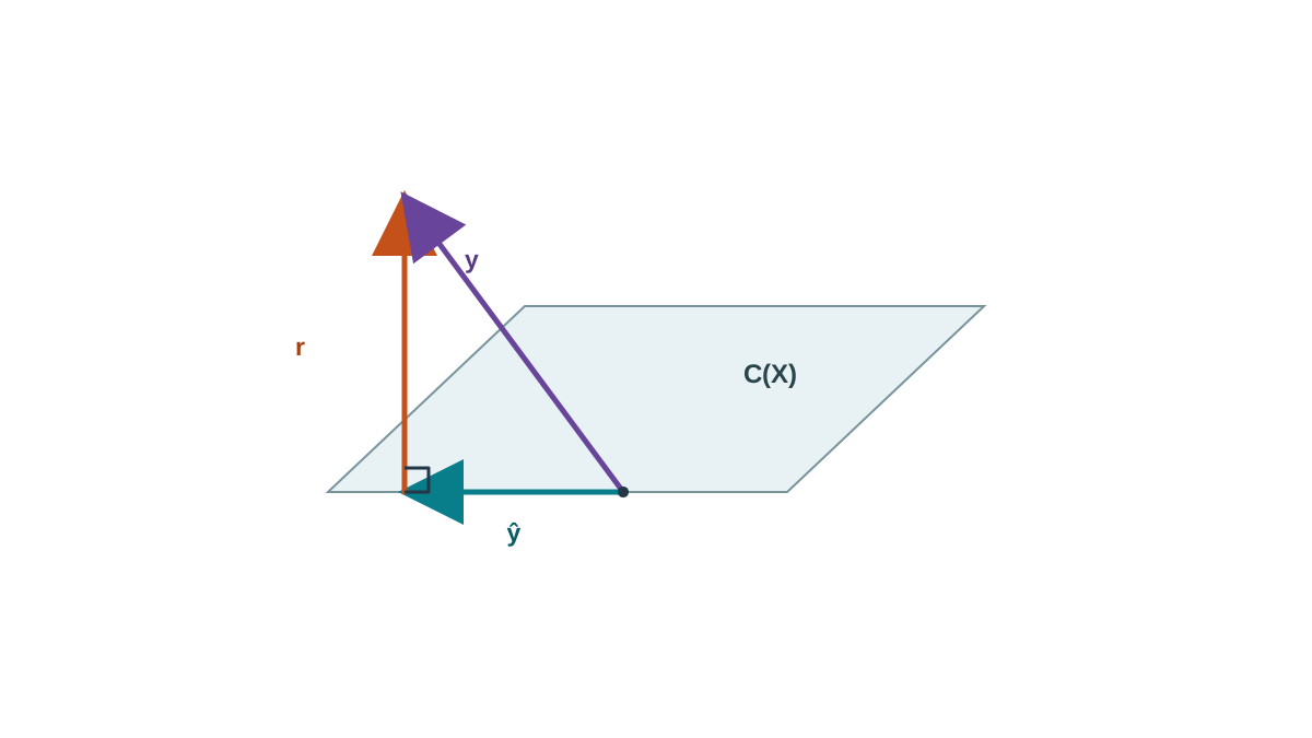
Let us derive it rather than assert it. Suppose $\hat{\beta}$ minimizes the objective. Pick any direction $u \in \mathbb{R}^p$ and consider moving along it: $\hat{\beta} + tu$. If $\hat{\beta}$ is truly the minimizer, then the objective at $t = 0$ cannot be beaten, so the function

has a minimum at $t = 0$. Write $r = y - X\hat{\beta}$. Then

This is a parabola in $t$ opening upward. Its minimum sits where the derivative vanishes:

Since $u$ was arbitrary, $(Xu)^\top r = 0$ for every $u$, which is the same as

Read that equation geometrically. $X^\top r$ is the vector of dot products between $r$ and each column of $X$. Setting it to zero says $r$ is orthogonal to every column, and therefore to every linear combination of columns — that is, to the entire column space.

The same condition falls out of the normal equations. Setting the gradient of $\|y - X\beta\|^2$ to zero gives $X^\top X \beta = X^\top y$, and rearranging yields $X^\top(y - X\hat{\beta}) = 0$. The normal equations are the algebraic shadow of the geometric fact. The geometry is the thing to remember; the algebra is how you compute it.

The Hat Matrix and the Two Orthogonal Pieces

The projection has a name and a matrix. Define

Then $\hat{y} = Hy$ and $r = (I - H)y$. This $H$ is the hat matrix, because it puts the hat on $y$.

Two properties do all the work. $H$ is symmetric ($H^\top = H$) and idempotent ($H^2 = H$). Idempotence is the algebraic statement that projecting twice is the same as projecting once — once you are on the plane, projecting again does not move you. The same holds for $I - H$, which projects onto the orthogonal complement.

Now the identity readers usually see quoted falls out in one line:

Fitted values and residuals are orthogonal because $H(I - H) = 0$: the two projection matrices target complementary subspaces. Nothing about your data entered that calculation.

Because the two pieces are perpendicular, the Pythagorean theorem applies to the vectors:

That is the vector-level version of the split between explained and unexplained variation you may have seen as sums of squares.

Common mistake: Reading $H$ as a property of your model's quality. $H$ depends only on $X$. Change $y$ to anything at all — random noise, a completely different process — and the identities still hold exactly. Orthogonality is a property of the fitting procedure, not of the fit.

Worked Example: Watch the Residuals Go Perpendicular

Let us make this concrete with numbers you can reproduce in a few lines of NumPy.

import numpy as np

# Four points, one predictor plus intercept
x = np.array([0.0, 1.0, 2.0, 3.0])
y = np.array([1.0, 3.0, 2.0, 5.0])

X = np.column_stack([np.ones_like(x), x])
beta, *_ = np.linalg.lstsq(X, y, rcond=None)

y_hat = X @ beta
r = y - y_hat

print("beta:", beta)
print("X^T r:", X.T @ r)      # should be ~[0, 0]
print("r . y_hat:", r @ y_hat)  # should be ~0

Run it and you will see X^T r print two values at machine precision — essentially zero — and r . y_hat likewise. The residuals are orthogonal to the intercept column and to the predictor column, and therefore to the fitted values.

Now the part that matters. Replace y with data that a straight line clearly cannot describe — say, points along a curve:

y_curved = np.array([1.0, 4.0, 9.0, 16.0])  # quadratic, not linear
beta, *_ = np.linalg.lstsq(X, y_curved, rcond=None)
y_hat = X @ beta
r = y_curved - y_hat

print("X^T r:", X.T @ r)      # still ~[0, 0]
print("r . y_hat:", r @ y_hat)  # still ~0

The identities hold exactly, to machine precision, even though the model is wrong. Plot the residuals against the fitted values and you will see a clear U-shaped pattern — the signature of a missing quadratic term. The orthogonality is intact; the model is still bad.

That is the central demonstration of this article. The angle tells you nothing. The shape tells you everything.

What Orthogonality Does Not Prove

This is where the geometry ends and statistics begins, and confusing the two is the most common error I see in intermediate learners.

The statement $r \perp \mathcal{C}(X)$ is a theorem about a minimization problem. It is true for any $y$, any full-rank $X$, and any solver that actually finds the minimum. It says nothing about:

• whether the true relationship between predictors and target is linear,
• whether the error variance is constant across observations,
• whether the errors are independent,
• whether you have omitted a relevant variable,
• whether the errors are normally distributed.

Those are claims about $\varepsilon$, the unobservable noise term, and they require assumptions you impose on top of the geometry. The geometric result is about $r$, the observable residual. They are different objects, and the identity connecting them only holds under a correctly specified model.

Note: When $X$ is rank-deficient — for example, two identical predictor columns — $\hat{\beta}$ is not unique. The fitted values $\hat{y}$ and the residuals $r$ still are, because they depend only on the column space, not on which basis you chose for it. Orthogonality survives; coefficient interpretation does not.

The practical consequence is the one your residual-analysis workflow already told you: you must look at the shape of the residuals, not just their correlation with $\hat{y}$. That correlation is zero by construction. Plot $r$ against each predictor, against $\hat{y}$, and against observation order, and ask what structure survived the fit.

Where the Geometry Changes: Weighted and Nonlinear Least Squares

The clean perpendicular picture is a special case, and knowing when it stops applying keeps you from misapplying the intuition.

Weighted least squares minimizes $\|W^{1/2}(y - X\beta)\|^2$ for a weight matrix $W$. The residuals are orthogonal to the columns in the transformed space, not the original one. If you plot raw residuals against raw fitted values, the orthogonality you expect may not appear — and that is correct behavior, not a bug.

Nonlinear least squares minimizes $\|y - f(\beta)\|^2$ where $f$ is nonlinear in $\beta$. There is no global column space. At the solution, orthogonality holds between the residual and the columns of the Jacobian — the local linearization. Solvers like SciPy's leastsq expose this directly: the gtol parameter controls the desired orthogonality between the function vector and the Jacobian columns, and it is used as a convergence criterion. Orthogonality becomes something the algorithm enforces rather than something the geometry guarantees.

Total least squares measures the distance from each point to the fitted line along the shortest direction, not vertically. The residual is perpendicular to the fitted curve in the original coordinate space, which is a genuinely different geometry from ordinary least squares.

The takeaway: before you claim orthogonality, name the norm and name the space. The identity is only as meaningful as the objective it came from.

Reading Residuals With the Right Mental Model

Here is how I want you to use this.

Treat orthogonality as a sanity check on your computation, not as evidence about your model. If you compute $X^\top r$ and it is not essentially zero, something is wrong with your solver, your design matrix, or your arithmetic. That is a useful alarm. It is not a quality score.

When residuals show structure — curvature, a funnel, clusters — the fix is almost never a different solver. It is a different feature, a transformation, an interaction term, or a different model form. The solver did its job perfectly; it found the closest point in the subspace you gave it. If that subspace cannot represent the truth, no amount of numerical care will save you.

When residuals look random, remember that randomness is consistent with many unmodeled problems: omitted variables, heteroscedasticity, dependence between observations. A clean residual plot narrows the space of things that are obviously wrong. It does not certify that anything is right.

The angle is guaranteed. The shape is the evidence. Go refit a model you already have, verify $X^\top r = 0$ numerically, then plot $r$ against $\hat{y}$ and against each predictor. Ask what structure survived the projection — that is the question the geometry was never going to answer for you.