
Decompose the Brier Score Into Reliability, Resolution, and Uncertainty
Two forecasters can post the same Brier score and deserve opposite verdicts. One is honest but says almost nothing. The other is sharp but lies about its…

Key topics
Two forecasters can post the same Brier score and deserve opposite verdicts. One is honest but says almost nothing. The other is sharp but lies about its probabilities. A single number cannot tell you which one you are holding.
That is why the decomposition exists. The Brier score is the mean squared difference between your predicted probability and the 0/1 outcome, bounded in [0, 1], lower is better. It is a proper scoring rule: you minimize it by reporting your honest probability. But it fuses two different failure modes into one number — probabilities that do not match observed frequencies, and probabilities that never move away from the base rate. The decomposition pulls them apart.
This article works one stated grouped-probability decomposition and interprets its terms. It does not re-derive calibration curves or compare calibration methods. If you already know what a reliability diagram shows and why ranking and calibration are separate questions, you have the prerequisite. The job here is to compute the three terms by hand and read each one as its own diagnostic.
Why One Brier Score Cannot Answer Two Questions
Consider two forecasters on the same set of events.
Forecaster A always predicts the base rate. If 30% of outcomes are positive, A says 0.30 every time. A is perfectly calibrated in the aggregate — its stated probability matches the observed frequency. But A carries zero information. It never separates a high-risk case from a low-risk one.
Forecaster B is aggressive. It says 0.95 when it is confident and 0.05 when it is not, and it ranks cases well. But when it says 0.95, the event happens only 70% of the time. B is informative and badly miscalibrated.
Both can land near the same Brier score. A scores respectably by refusing to commit. B scores badly by committing and being wrong about the magnitude. The raw score treats these as similar. The decomposition does not.
The Brier score mixes two questions: are your probabilities honest? and do your probabilities separate cases? A third quantity — the difficulty of the problem itself — sets the reference both of them work against.
Knowledge check
Check your understanding
Answer this question before you continue.
Notation and the Grouped Setup
Define the pieces before using them.
You have forecasts. Each forecast has a predicted probability and a realized binary outcome . The raw score is:
Now group. Bucket the forecasts into bins by predicted probability. For bin :
- — number of forecasts in the bin
- — the bin's probability value (the probability shared by forecasts in that bin)
- — the observed frequency, i.e. (number of 1s in bin ) /
Define the overall base rate as the mean of all outcomes across all forecasts.
Note: The three-term identity is exact only when every forecast inside a bin shares the same probability value. With real-valued probabilities, binning introduces within-bin variation, and the three terms no longer sum exactly to the raw score. Extra within-bin terms appear. This is a known limitation, not a rounding error — I will return to it.
The bin count is a choice, and it changes the answer. More on that below.
Knowledge check
Check your understanding
Answer this question before you continue.
The Three Terms, One at a Time
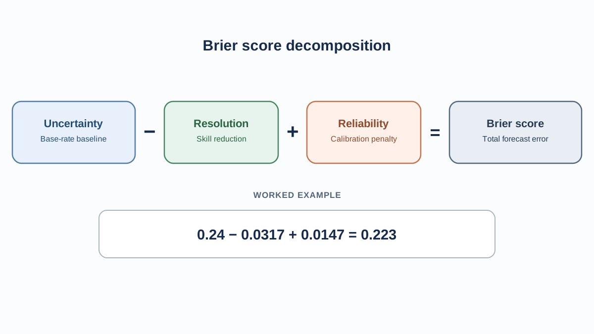
Each term gets its own mechanism.
Reliability is the -weighted average of . It measures how far your stated probabilities drift from observed frequencies. If you say 0.80 and the event happens 80% of the time in that bin, the term contributes nothing. Lower is better. A perfectly calibrated forecaster has reliability zero.
Resolution is the -weighted average of . It measures how far the outcome rate inside each bin moves away from the base rate. If every bin has the same outcome rate as the overall base rate, resolution is zero — the model separates nothing. Higher is better. A forecaster that always predicts the base rate has resolution zero by construction.
Uncertainty is . It depends only on the outcome prevalence, not on the model at all. It is maximal at a 50/50 base rate and zero when the outcome never or always occurs. No model can change it.
The identity:
Read the signs carefully, because this is where readers get it wrong. Miscalibration adds error. Informative separation subtracts error. Uncertainty is the score of the uninformative base-rate forecast — the reference point that resolution improves on and reliability penalizes.
That reference framing matters. Uncertainty is not a floor on the score you can achieve. A model that is perfectly calibrated and perfectly separating scores zero, even when the outcome is genuinely uncertain. What uncertainty tells you is how much a base-rate-only forecast would score on this problem. Resolution is the credit you earn by beating that baseline; reliability is the penalty you pay for probabilities that do not match reality.
Knowledge check
Check your understanding
Answer this question before you continue.
A Worked Example on Ten Forecasts
Ten forecasts, grouped into three bins.
| Bin | 1s | |||
|---|---|---|---|---|
| 1 | 0.20 | 4 | 1 | 0.25 |
| 2 | 0.50 | 3 | 1 | 0.333 |
| 3 | 0.80 | 3 | 2 | 0.667 |
Total outcomes: out of 10, so .
Raw Brier score. Using the individual forecasts (bin probability applied to each member):
- Bin 1: four forecasts at 0.20, one outcome 1 and three outcomes 0. Errors: once, three times. Sum .
- Bin 2: three forecasts at 0.50, one outcome 1 and two outcomes 0. Errors: once, twice. Sum .
- Bin 3: three forecasts at 0.80, two outcomes 1 and one outcome 0. Errors: twice, once. Sum .
Total . Divide by : BS = 0.223.
Reliability.
Resolution.
Uncertainty.
Verify the identity.
That matches the raw score. The arithmetic closes.
Interpretation. The score is 0.223. A base-rate-only forecast on this problem would score 0.24, so this model beats the baseline by 0.0317 through resolution and gives back 0.0147 to miscalibration. The net gain over the baseline is small but real. Reliability is low, so the probabilities are roughly honest. Resolution is modest, so the bins separate, but not dramatically. The model is doing something, just not much.
A recalibrated variant. Suppose you recalibrate so each bin's stated probability matches its observed frequency: bin 1 becomes 0.25, bin 2 becomes 0.333, bin 3 becomes 0.667. The bin ordering is unchanged, so resolution stays at 0.0317. Reliability drops to zero. The new score is . The improvement came entirely from the term you targeted. That is the check you want: move one term, confirm the score moved for the reason you intended.
Knowledge check
Check your understanding
Answer this question before you continue.
What Each Term Is Allowed to Claim
The decomposition is a diagnostic, not a verdict. Each term licenses a specific claim.
Reliability isolates systematic over- or under-confidence. It is the term recalibration is designed to reduce. If reliability is large relative to resolution, your probabilities are drifting from reality in a way a calibration step can address.
Resolution reflects whether the model separates high-risk from low-risk cases. If resolution is near zero, the model is not distinguishing anything — it is a base-rate machine. No amount of recalibration fixes that. You need better features or more model capacity.
Uncertainty is a property of the problem, not the model. This has a sharp practical consequence: comparing raw Brier scores across datasets with different base rates compares difficulty as much as skill. A score of 0.15 on a 50/50 problem and a score of 0.15 on a 5% base-rate problem are not the same achievement.
Common mistake: Assuming a low Brier score means good calibration. It does not. A model can score low by being well calibrated, or by being uninformative on an easy problem. High resolution does not guarantee usable probabilities either — a sharp model can be sharp and wrong.
The components are not independently optimizable. Driving reliability to zero does not automatically improve the score, because recalibration can flatten the probabilities and reduce resolution. Pushing resolution up can raise reliability if the model becomes overconfident. The terms trade against each other. Report the decomposition alongside a calibration view, not instead of it.
Where the Decomposition Breaks Down
The three-term reading is trustworthy only inside its assumptions.
Bin-count sensitivity. Reliability and resolution both change as you change the number of bins. Uncertainty does not. With too few bins, both terms are understated — a single bin forces resolution to zero by definition. With too many bins, each bin holds too few forecasts and the observed frequencies become noisy. The bin count is a modeling choice, and it moves the answer.
Within-bin variation. When forecasts inside a bin differ, the identity is no longer exact. Additional within-bin variance and covariance terms appear, and the clean three-term sum breaks. If you stratify on distinct probability values instead of binning, the within-bin terms vanish and the identity holds exactly.
Small samples per bin. Noisy observed frequencies inflate apparent reliability and resolution. A bin with three forecasts tells you almost nothing about the true conditional frequency.
It describes the past, not the future. The decomposition describes the forecasts you scored. It says nothing about distribution shift or whether the probabilities will stay calibrated on new data.
When not to lean on it. Very small evaluation sets, heavily imbalanced outcomes where uncertainty is near zero, and settings where you only need a ranking rather than a probability. If you never act on the probability magnitude, the decomposition is measuring something you do not use.
A Practical Reading Routine
Turn the decomposition into a repeatable sequence.
- Collect aligned pairs. Gather each predicted probability and its realized outcome from a held-out set, not from training data.
- Compute the raw Brier score. This is your headline number.
- Bin the probabilities. Choose a bin count you can defend, then compute reliability, resolution, and uncertainty.
- Read the terms in order. Is the score dominated by miscalibration, by weak separation, or is it close to the base-rate baseline?
- Choose the next action from the dominant term. Reliability large relative to resolution: recalibrate. Resolution near zero: revisit features or model capacity. Score near the base-rate baseline: the model is adding little, so the bottleneck is the model, not the problem's difficulty.
- Re-run after any change. Confirm the improvement came from the term you intended to move.
My rule is simple: read reliability first, resolution second, and treat uncertainty as the baseline you are trying to beat. Reliability tells you whether you can trust the number. Resolution tells you whether the number is worth trusting. Uncertainty tells you what "worth trusting" costs on this problem.
The same grouped reasoning extends to multi-class problems through the ranked probability score, where the decomposition generalizes and the same three roles reappear. The natural next step is to apply this routine to your own held-out predictions and pair the decomposition with a calibration plot — the plot shows you the shape of the miscalibration, and the reliability term tells you how much it costs.
Knowledge check
Final check
Finish the article by checking the ideas you just learned.
References
Build stronger machine learning foundations
Use structured resources to connect theory, scikit-learn workflows, and evaluation practice.


